
Miao Yu, Yaolu Zhang, Zechen Xu, Yutong He. Signal feature extraction method based on MEEMD-HHT for distributed optical fiber vibration sensing system[J]. Infrared and Laser Engineering, 2021, 50(7): 20210223
- Infrared and Laser Engineering
- Vol. 50, Issue 7, 20210223 (2021)
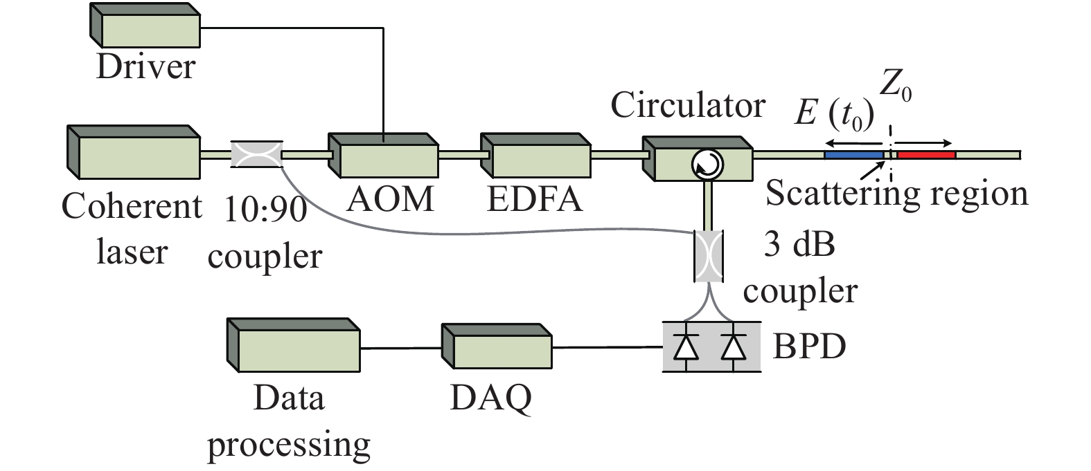
Fig. 1. Experimental device diagram of distributed optical vibration sensing system
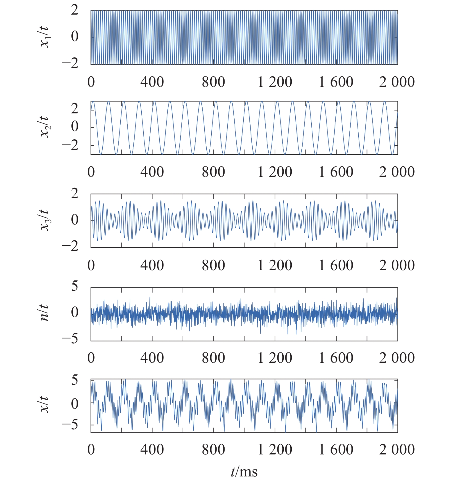
Fig. 2. Vibration simulation signal and the composition of the time-domain waveform
Fig. 3. EMD decomposition results of simulation signal
Fig. 4. CEEMD decomposition results of simulation signal
Fig. 5. MEEMD decomposition results of simulation signal
Fig. 6. Reconstruction error of three decomposition methods
Fig. 7. Phase-time change curves of vibration signals of different frequencies demodulated by the system
Fig. 8. Hilbert spectrum after three kinds of empirical mode decomposition and Hilbert transforn of vibration signal whose frequency is 100 Hz
Fig. 9. Hilbert spectrum after three kinds of empirical mode decomposition and Hilbert transforn of vibration signal whose frequency is 200 Hz
Fig. 10. Hilbert spectrum after three kinds of empirical mode decomposition and Hilbert transforn of vibration signal whose frequency is 50 Hz,200 Hz,350 Hz
Fig. 11. Hilbert spectrum after three kinds of empirical mode decomposition and Hilbert transforn of vibration signal whose frequency is 150 Hz,250 Hz,450 Hz
Fig. 12. Marginal spectra of three decomposition methods on different frequencies
|
Table 1. Permutation entropy of eight signals
|
Table 2. Each method index
|
Table 3. Frequency extraction accuracy test
|
Table 4. Three methods of experimental results

Set citation alerts for the article
Please enter your email address
© Copyright 2018-2021 | Chinese Laser Press. All Rights Reserved 沪ICP备15018463号-20