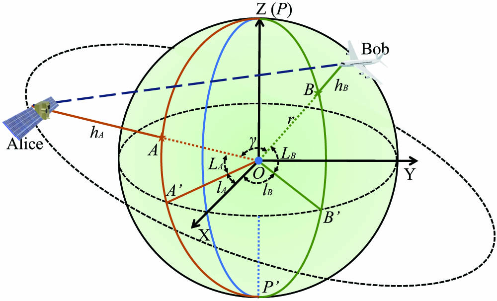
Fig. 1. Schematic diagram of satellite and aircraft in the WGS-84 coordinate system.

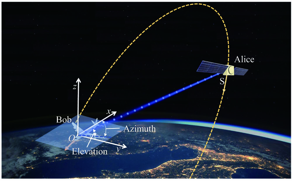
Fig. 2. Schematic diagram of downlink satellite-to-aircraft QKD in the spherical coordinate system based on the aircraft. The satellite (Alice) flies in a certain orbit above the receiving aircraft (Bob).

Fig. 3. Schematic diagram of the distance between the BL and receiver telescope.

Fig. 4. Diagram of the satellite-to-aircraft QKD performance evaluation.

Fig. 5. Schematic diagram of photon aberrations evaluation. The photons propagate through the BL to the receiver telescope, and the wavefront aberration can be calculated by the ray-tracing method.

Fig. 6. Evaluated density field distribution of the DLR-F6 BL. The dimensions of the BL are 500mm×500mm×50mm.

Fig. 7. Total loss over the different incident angles. Here they are α = 0°, 90°, 180°, 270°.

Fig. 8. Schematic diagram of satellite-to-aircraft QKD from 12:00 on May 29, 2022, to 12:00 on June 5, 2022. The yellow arrow indicates the direction of flight of the aircraft.

Fig. 9. (a) Total loss in the satellite-to-aircraft QKD scenario; (b) estimated QBER over the communication time; (c) secure key rate over the communication time. The value of X₀ is 66 mm and the aircraft flights toward the south. The intensity of signal states is 0.8, and the intensity of decoy states is 0.1.

Fig. 10. (a) Total loss in the satellite-to-aircraft QKD scenario; (b) estimated QBER over the communication time; (c) secure key rate over the communication time. The value of X₀ is 66 mm and the aircraft flights toward the east. The intensity of signal states is 0.8, and the intensity of decoy states is 0.1.

Table 1. Parameters of Airborne QKD