Rumao Tao, Xiaolin Wang, Hu Xiao, Pu Zhou, Lei Si, "Coherent beam combination of fiber lasers with a strongly confined tapered self-imaging waveguide: theoretical modeling and simulation," Photonics Res. 1, 186 (2013)
Copy Citation Text
Coherent beam combination (CBC) of fiber lasers based on self-imaging properties of a strongly confined tapered waveguide (SCTW) is studied systematically. Analytical formulas are derived for the positions, amplitudes, and phases of the self-images at the output of a SCTW, which are important for quantitative analysis of waveguide-based CBC. The formulas are verified with numerical examples by a finite difference beam propagation method (FDBPM) and the errors of the analytical expressions are studied. This study shows that the analytical formulas agree well with the FDBPM simulation results when the taper angle is less than 1.4° and the phase distortion is less than . The relative errors increase as the taper angle increases. Based on the theoretical model and the FDBPM, we simulated the CBC of fiber laser array and compared the CBC based on the tapered waveguide with that based on the nontapered one. The effects of input beam number, aperture fill factor, and taper angle on the combination performance have been studied. The study reveals that a beam which has near-diffraction limited beam quality () and a single beam without side lobe in the far field can be achieved with tapered-waveguide-based CBC. It is shown that beam quality depends on input beam number, aperture fill factor, and taper angle. There exists a best fill factor which will increase as input beam number increases. The tolerance of the system on the fill factor and the taper angle is studied, which is and , respectively. The results may be useful for practical, high-power fiber laser systems.
Due to high conversion efficiency, excellent beam quality, convenient heat management, and compact configuration of fiber lasers [1], fiber lasers have wide applications, i.e., in industrial processing and optical communication. With the development of high-power laser diode pump technology and double-clad fiber production crafts, the output power of fiber lasers has been increasing rapidly in recent years. However, due to nonlinear effect, facet fracture, and thermal lens [2], the ultimate output power of a single fiber laser cannot increase unrestricted. A promising approach to overcome this difficulty is coherent beam combination (CBC) of multiple fiber lasers, which can achieve a high-power laser beam with good beam quality while maintaining excellent heat-managing capability [3–10]. To date, most of the prevalent architectures for CBC of fiber lasers have involved free-space phased arrays that incorporate multiple tiled emitters. A unity fill factor is required for free-space phased array architecture to ensure the far-field beam quality [4–10]. However, this is too difficult for practical engineering and much of the power in the central lobe is diverted to side lobes. Alternative solutions based on filled-aperture designs, such as those based on diffractive optical elements (DOEs) [11], coherent polarization beam combination (CPBC) [12], and reimaging assisted phased arrays (REAPAR) [13,14], offer much better combining efficiencies and thus reduce side lobes in the far field compared with the aforementioned architectures. The REAPAR architecture, based on the self-imaging properties of waveguides, was first developed by Christensen and Koski for CBC in planar waveguides [13]. Recently it was reported that, based on fiber laser array, the REAPAR technology has been extended to two-dimensional (2D) waveguides and successfully implemented at high power levels [14]. One potential complication during the implementation of the aforementioned configuration is the very close packing of the laser array, which will be on the order of hundreds of micrometers. Tapered waveguide is a special kind of waveguide which, expanding the launch aperture while maintaining the output aperture, can be used in CBC and provide convenient operation with large input beam spacing [13]. However, to the best of our knowledge, the theoretical model to analyze the tapered-waveguide-based CBC of fiber lasers has not been reported.
In the present paper, we discuss the self-imaging properties of fiber lasers in a strongly confined tapered waveguide (SCTW) and its potential application in CBC of fiber lasers. Analytical formulas are derived for the positions, amplitudes, and phases of the self-images at the output of a SCTW. A finite difference beam propagation method (FDBPM) is used to verify numerically the analytical expressions. Base on the analytical results and the FDBPM, the tapered-waveguide-based CBC of the fiber laser array is investigated, and the CBC results based on a tapered waveguide are compared with that based on a nontapered one. The combining performance of the system is also investigated, followed by some instructive discussions.
2. THEORETICAL MODEL
A. System Introduction
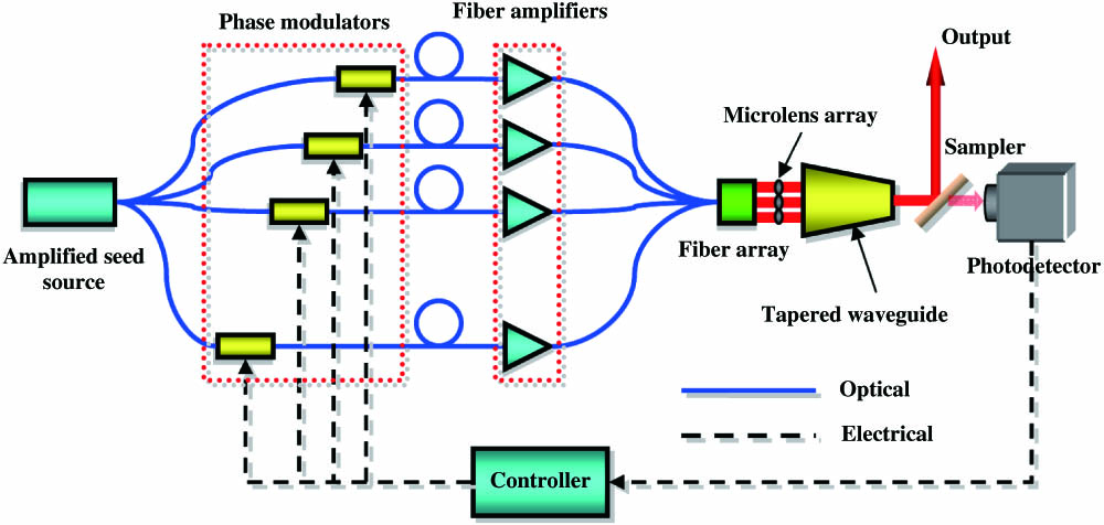
The CBC system based on a tapered waveguide is depicted in Fig. 1. The beams emerging from amplified seed source pass through phase modulators, and then through fiber amplifiers. The amplified beams are coupled into the transport fibers and form a fiber array, which passes through a microlens array. The microlens array is used to focus the beams into the combining tapered waveguide. A small portion of the combined output laser is picked off with a high-reflector and detected with a photodetector. The photodetector output is sent to the controller and is used as a closed-loop feedback signal to control the phase modulators. Then the amplified beams are coherently combined into one single beam.
Sign up for Photonics Research TOC. Get the latest issue of Photonics Research delivered right to you!Sign up now
Figure 1.Schematic diagram of the waveguide-based CBC system.
For the sake of simplicity, a tapered waveguide of homogeneous refractive index with symmetric cladding (as shown in Fig. 2) is considered, which provides one-dimensional self-imaging. is the input width, is the output width, and is the taper angle between the axis and the tapered side of the waveguide (if , is positive; on the contrary, is negative). Figure 3 shows the amplitude distributions in SCTW in the case of a Gaussian beam input (which is a good approximation for fiber lasers). In the numerical simulation, the origin of the axis is taken to be at the center, which is taken to be on the one side as shown in Fig. 2 in derivation. We denote the characteristic distance of propagation, where the input amplitude profile is reconstructed (with some aberrations) in a loss-free, straight waveguide, as . It can be seen from Fig. 3 that, if the laser is incident at the offset position, the self-image can only happen at ; however, self-image can be achieved at when the laser is incident at the axially aligned position. It is advantageous when the fiber laser is incident at the axially aligned position since it can shorten the imaging length of the waveguide, which can save space and make the application more compact, so we mainly focus our attention on the latter situation.
Figure 2.Schematic diagram of a tapered waveguide.
The theory is developed for arbitrary symmetric input light distribution and for a 2D tapered waveguide. However, with the effective index method, which is reasonably accurate for strongly guided modes [15], the practical 3D problem can be reduced to two dimensions. The present results are relevant for square and rectangular self-imaging produced by 3D waveguides of square or rectangular cross sections [16,17]. The application of waveguide to coherent combining of lasers is the reverse use of the self-imaging effects [13,14]. We consider the imaging of a symmetric beam through a 2D tapered waveguide to simplify the discussion. For a strongly confined waveguide, guided modes are almost completely confined within the waveguide and their lateral mode profiles contain an integer number of half-periods within the waveguide [17,18]. Defining the incident plane as the original plane and using a spatial Fourier decomposition, the incident light distribution can be rewritten as a superposition of the infinite number of strongly even guided eigenmodes with the coefficients : The symmetry properties of the input light distribution and the axially aligned incident properties are used to obtain Eq. (1). The strongly guided eigenmodes at plane have the form of where is the mode number and is the active width of the waveguide. is equal to the physical thickness , which is slightly corrected at both sides by the Goos–Hahnchen penetration depth in the cladding of index [15,16,18]: where for TE polarization, for TM. is the index of the waveguide.
The transverse propagation constants are and the corresponding longitudinal propagation constants are
With paraxial approximation, one can obtain or where is the propagation constant in vacuum, .
According to Eq. (6c), we can conclude that if the two lowest-order modes (zero-order and second-order) are coupled, all the other higher modes will fulfill the couple condition. If we set as the shortest coupling length (self-imaging length), then the following relation can be established as
Substituting Eq. (3) into Eq. (7), self-imaging length can be expressed as where .
The output field at plane (the subscript denotes the number of the self-images, which means the number of the fiber lasers that can be combined by the waveguide when the waveguide is used for CBC) is
Substituting Eqs. (5) and (2) into Eq. (9), one can achieve
Equation (10b) can be calculated recursively:
Then the coefficient is introduced, which is defined as with According to Eqs. (12) and (13d), .
Using Eqs. (13a)–(13c), one can obtain
Recalling the periodicity of the summands, the coefficients can be written as Comparing Eq. (11) with Eq. (15), only if one of the following relations is fulfilled: or can the following relationship be established:
Replacing the summation index of the sum with , the above expression can be written as
Inserting Eq. (15) into Eq. (9), one can obtain Then The output field distribution can be rewritten as
According to Eq. (1), Eq. (20) can be rewritten as
According to Eq. (21), a sum of images with equal amplitudes numbered by are obtained. Due to the fact that the waveguide is tapered, the images at the output of the waveguide () are different from the initial input field (). Setting , the relations for nontapered waveguides can be obtained. Equations (3), (8), (13), and (16) are the main results obtained in this manuscript, which are the essential condition to realize the SCTW-based CBC. Combined with a FDBPM, the waveguide-based CBC of fiber lasers can be studied numerically.
3. NUMERICAL RESULTS
To verify the formulas derived in Section 2, numerical simulation examples are presented. We take the values determined by numerical techniques as numerically exact [19] and use them in the comparison to justify our formulas by numerical examples. A FDBPM [20,21] is used to simulate the light propagation in the tapered waveguide section. The computational core of our simulation program is described in [20,21], which has been improved based on the method described in [22–25] and referenced therein. The simulation results obtained with the FDBPM can provide reliable accuracy [26,27] for comparison. In the FDBPM simulation, we choose the discretization sizes μ. A relative error is defined to characterize the length error of our analytical model, which is expressed as where is the waveguide length predicted by our analytical model and is the waveguide length obtained through FDBPM. The is obtained by maximizing the power in the bucket (PIB) criterion, which indicates how much energy is transferred to the main lob and is defined as where is the radius of the bucket. With the predicted by Eq. (16), we just need to analyze the simulation results near to find more accurate results, , which are time-saving and useful to reduce the cost in practical application.
We consider a SCTW with μ, , and . The waveguide is situated in air, i.e., ; μ is taken here. Gaussian beams with waist width of 5 μm are launched at . The relative small size of the waveguide and beam size compared to that used in the real experiments are due to the limitation of computation resources. Figure 4 shows the field distribution of the waveguide by the FDBPM simulation with “transparent” boundary conditions [28,29]. Equation (7) predicts that the self-imaging length is μ and the self-imaging length given by the FDBPM simulation results is μ [see Fig. 4(c)], with . Choosing with incident position and phase relation indicated by Eq. (13), we obtained μ, and the self-imaging length given by the FDBPM simulation results is μ [see Fig. 4(d)], with . Figures 4(e)–4(h) give the field distribution at the simulated length. From Figs. 4(e) and 4(g), we can obtain that the self-imaging of the input laser beam is obtained with some degree of compression; from Figs. 4(f) and 4(h), the combining of the two Gaussian beams is achieved, which proves the accuracy of the incident position and phase relation indicated by Eq. (13). One can obtain from Figs. 4(g)–4(h) that, within the main lobe area, the phase difference between our analytical model (plane) and the simulation is negligible (less than ). It can be also found from Figs. 4(a) and 4(b) that the self-imaging properties of the tapered waveguide are distorted as indicated in Eq. (21), and the combined performance is degraded.
Figure 4.Field distribution at the output of the SCTW. (a), (c), (e), and (g) are for the self-imaging of the laser beam; (b), (d), (f), and (h) are for the combination application.
For perfect self-imaging, the field of the self-imaging beam is the same as that of the input beam from Eqs. (8) and (21). However, it reveals in Figs. 4(e)–4(h) that the fields of the laser beam are distorted. The phase distributions of the self-imaged beam fluctuate within a narrow range while the phase distributions of the input beam are plane. This can be understood easily from the analytical derivation. For complete mode decomposition in Eq. (8), we need an infinite number of guided modes totally confined within the waveguide. The resulting approximation errors have been investigated and are negligible for nontapered, strongly confined structures [16]. However, due to the taper of the waveguide, the confining capacity of the SCWT becomes weakened and more high-order modes leak out of the waveguide, which result in larger approximation errors and imperfect combining (imaging) performance.
To further study the effects quantitatively, we simulated the combining of two fiber lasers in SCWT with different taper angles. The parameters are listed in Table 1 and the results are shown in Fig. 5. It is shown that the distortion is negligible when and perfect combining performance can be achieved. The distortion of the field at the output of the SCWT increases with the taper angle, and the power in the main lobe is reduced to 76% when (). This is due to the fact that more high-order modes leak out with larger taper angle, which results in deterioration of the combining (imaging) performance. To ensure more than 90% of the energy contained in the main lobe, the taper angle must be set to less than 1.4° (). Within the main lobe area, the phase distribution for the tapered waveguide is nearly plane and the phase fluctuation is less than when . From Figs. 4 and 5, one sees that our analytical formulas agree well with the FDBPM simulation results when and the deviation becomes larger as the taper angle increases. Our analytical model is accurate for small taper angles, i.e., , and can be used to design the SCWT and the fiber laser array in waveguide-based CBC systems, which is useful in practical application.
Figure 5.Field distributions at the output of the SCTW for different taper angles. (a), (c) Amplitude distribution and (b), (d) Phase distribution.
Based on our analytical formulas and the FDBPM, the combining of fiber laser array (shown in Fig. 6) in the 3D square-cross tapered waveguide is simulated with different . The waist diameter of the laser beam is 5 μm. The relative phase and positions in the input plane are shown in Table 2, and the other parameters are taken to be the same as those in Fig. 4. The parameters of the waveguide are listed in Table 3. The fiber lasers can be effectively combined provided the relative phase and incident position indicated in Eq. (13) are fulfilled. From Fig. 7, we can conclude that, with larger taper angle, the output beam is more compressed and more energy is diverted into the side lobes.
B. Combination Based on Nontapered Waveguides and Tapered Waveguides
The combining of fiber laser arrays based on tapered waveguides is compared with that based on nontapered waveguides in this section. The output size of the waveguides is taken to be the same. Beam waist radius of each fiber laser is 2.5 μm with power . If a nontapered waveguide is adopted to combine the array laser beams, we can determine that μ. Figure 8 presents the output intensity distribution of fiber lasers based on different waveguides. It reveals that, with the same size output port, the peak energy of the combined beam is higher for CBC based on a tapered waveguide, which is due to the taper of the waveguide.
Figure 8.Transverse intensity distribution of fiber lasers.
The results of two kinds of CBC systems are listed in Table 4 for comparison. It indicates that, compared with planar waveguides, larger input size can be achieved using tapered waveguides, which is meaningful for coupling the fiber laser array into the waveguide but is achieved at the cost of waveguide length. In the practical application, we should choose waveguide based on a practical situation.
For applications such as energy transmission, the beam quality of the combined beam is a key parameter to our concern. The well-known parameter is taken as the characteristic parameter to analyze the combination performance of the system which, for the 2D case, is defined as [30] with
Defining a fill factor to characterize the filling of the input part of the waveguide, we can get the results in Fig. 9. For the sake of simplicity, we consider the 1D array. The parameters of the waveguide are taken to be the same as in Fig. 4, except for the variable parameters. From Fig. 9(a), we can conclude that there exists an optimal , which corresponds to a best input beam waist. It proves that near-diffraction limited beam quality () is obtained. We define a tolerance to ensure that the value of the is less than 1.43, and the tolerance on fill factor is . It is shown, by comparing the results in Figs. 4(f) and 9(b), that the phase distortion of the output field can be mitigated by optimization of the fill factor . The far-field intensity distribution [Fig. 8(c)] is obtained by propagating the near field in free space using the Fast Fourier Transformation method [31,32]. It reveals that although the near field has side lobe, one single beam without side lobes can be achieved in far field by optimization of the fill factor.
Figure 9.Optimal designation of the system and the results. (a) as a function of , (b) near-field distribution for the optimum , and (c) far-field intensity distribution for different .
Figure 10 gives optimum for different numbers of lasers. One can see that, with input beam number increasing, the optimal increases and the beam quality of the combined beam decreases: the optimum is 1.84 for and 2.26 for . This is due to the fact that more high-order modes are generated in the waveguide (tapered or nontapered) with larger , which leak out and result in deterioration of the beam quality.
Figure 10. as a function of for different beam array.
Figure 11 reveals the influence of the tapered angle. The beam waist width is 7.5 μm. It shows that, with larger taper angle, the beam quality of the combined beam degrades and the length of the SCWT becomes short. Although the best beam quality () can be obtained when nontapered waveguides are used, the length of the waveguide (μ) is one half longer than that of the tapered waveguide (, μ), which may prevent a compact system configuration. One can conclude that the use of tapered waveguide can result in a compact configuration with moderate degrading of the beam quality. It also shows that the tolerance on the taper angle is .
Although the manufacturing of 3D tapered waveguides is not easy, the designation of 2D tapered waveguides is realizable. Figure 12 shows the combination based on a 2D tapered waveguide. The 2D waveguide is approximated by a rectangular cross with the short side (in the direction) being μ and the long side (in the direction) being 50 μm. The waveguide is shown in Fig. 12(a). The long side is far longer than the short side and the longer side of the waveguide has no taper while the short side tapers gradually. The parameters are taken as . The waist width of two Gaussian beams is 0.5 μm. Figure 12(c) shows the two fiber laser beams combined into a single laser beam. In practice, the aforementioned approach can be realized by using two metal plates with dielectric coating or glass plates with grazing incidence, high-reflection coating.
Figure 12.Combining based on 2D SCWT. (a) Schematic diagram of a 2D tapered waveguide, (b) intensity distribution of input laser beams, and (c) intensity distribution of output laser beams.
The actual order of the waveguide is hundreds of micrometers in the experiments. Hence, modeling the real waveguide requires at least one order of magnitude more computational time and memory than the modeled waveguide, which is beyond the computer resources in our lab for the time being. We are working to improve and optimize the computer programs to study the waveguide with the size in the experiment in the future. The conclusions obtained in the simulations are instructive for real experiments.
4. CONCLUSIONS
In this paper, we have presented a rigorous analysis for the self-imaging properties of fiber lasers in a SCWT and derived some analytical formulas for the positions, amplitudes, and phases at the output of the waveguide. Numerical simulation has been carried out to verify our analytical formulas. The results agree well with the predication of our analytical formulas when the taper angle is less than 1.4° and the phase distortion resulting from the taper of the waveguide is less than . The model is useful in designing and performance analyzing in the following ways:
It can predict the combing length (self-imaging length) of the tapered waveguide with error less than 1%, which is meaningful for saving time during designing the waveguide.
It can provide the phase relationships between the input laser beams and incident positions of the laser beams on the input part of the waveguide, which is useful in simulation of waveguide-based CBC based on beam propagation method.
It provides a direct insight of the CBC of laser beams based on tapered waveguide and proves this novel method theoretically.
Based on our analytical formulas and the FDBPM, we simulated the CBC of fiber lasers based on waveguide, and the effects of input beam number, aperture fill factor, and taper angle on the combination performance have been investigated. The engineering realization of such a configuration is discussed. It shows that this novel approach can achieve a high beam quality output beam (). If the output size is fixed, with larger taper angle, larger input size can be obtained; if the input size is fixed, shorter length of the waveguide and more compact system configuration can be obtained with larger taper angle. There exists an optimum fill factor . With input beam number increase, the optimum fill factor will increase and the beam quality will degrade. Although the near field distribution has a multilobe configuration, one single beam can be achieved in the far field. The tolerance of the system on the fill factor and the taper angle is studied, which is and . The CBC based on waveguide can be realized in 2D waveguide effectively. In practical application, we should choose and design waveguides based on the practical situation and take beam quality, system compaction, and cost into consideration.
ACKNOWLEDGMENTS
Acknowledgment. This project was supported by Innovation Foundation for Excellent Graduates in National University of Defense Technology under grant B120704.
[8] L. Liu, M. A. Vorontsov, E. Polnau, T. Weyrauch, L. A. Beresnev. Adaptive phase-locked fiber array with wavefront phase tip-tilt compensation using piezoelectric fiber positioners. Proc. SPIE, 6708, 6708K(2007).
[23] Y. Chung, N. Dagli. Modeling of guided-wave optical components with efficient finite-difference beam propagation methods. Antennas and Propagation Society International Symposium, 248-251(1992).
[24] C. Vassallo. Optical Waveguide Concepts(1991).
Rumao Tao, Xiaolin Wang, Hu Xiao, Pu Zhou, Lei Si, "Coherent beam combination of fiber lasers with a strongly confined tapered self-imaging waveguide: theoretical modeling and simulation," Photonics Res. 1, 186 (2013)