For fluorescence molecular tomography (FMT), image quality could be improved by incorporating a sparsity constraint. The L1 norm regularization method has been proven better than the L2 norm, like Tikhonov regularization. However, the Tikhonov method was found capable of achieving a similar quality at a high iteration cost by adopting a zeroing strategy. By studying the reason, a Tikhonov-regularization-based projecting sparsity pursuit method was proposed that reduces the iterations significantly and achieves good image quality. It was proved in phantom experiments through time-domain FMT that the method could obtain higher accuracy and less oversparsity and is more applicable for heterogeneous-target reconstruction, compared with several regularization methods implemented in this Letter.
Fluorescence molecular tomography (FMT) based on fluorochrome emission is capable of detecting in-vivo biological activities[1] and it is a sensitive functional imaging method that could quantitate fluorochrome concentrations at femtomolar levels[2]. However, due to its limited penetration in biological tissues, there are not many clinical applications of FMT but instead extensive applications in drug development[3,4] and cancer studies like the tumorigenicity study of glioblastoma xenografts in immunodeficient mice[5]. But it may be applied to imaging of the human wrist like in photoacoustic tomography[6].
Time-domain (TD) FMT utilizing pulsed excitation sources is one of the three approaches in FMT while the other two are continuous-wave (CW) FMT utilizing steady excitation sources and frequency-domain (FD) FMT utilizing modulated excitation sources. Fluorescence yield and fluorescence lifetime are the two primary parameters while lifetime is proved an excellent probe for local micro-environmental sensing[7]. Simultaneously recovering the fluorescent yield and lifetime distributions is only possible in TD-FMT and there are methods developed for that purpose[8,9]. Moreover, only for TD-FMT, it is possible to use early photons to achieve higher spatial resolution and stability[10,11].
Because of the strong scattering of the light in biological tissues, the reconstruction of FMT would be extremely ill-conditioned, limiting the quality of the reconstructed images. To improve the image quality, a conventional way is to incorporate a sparsity constraint in the inverse problem, adopting regularization methods such as Tikhonov regularization and L1-norm regularization. Although it is straightforward to utilize Lp-norm () regularization, the non-convex Lp-norm regularization could not be directly used in FMT reconstruction. But by applying a certain strategy, non-convex Lp-norm regularization could be solved by transferring into L1-norm to achieve better sparsity[12–14]. Among these, Tikhonov regularization is widely used and can be easily solved by iterative algorithms, while its solution is usually not sparse enough. However, according to our previous work[15], with a large number of iterations, an iterative Tikhonov regularization method that projects negative values to zero in each iteration could achieve sparse reconstruction results not worse than other regularization methods.
Sign up for Chinese Optics Letters TOC. Get the latest issue of Chinese Optics Letters delivered right to you!Sign up now
By studying how zeroing strategy achieves sparsity in the solutions, in this Letter, a Tikhonov-regularization-based projecting sparsity pursuit method (PrSP-Tk) is proposed that can achieve a better image quality than the Tikhonov regularization method with zeroing strategy (zeroing-Tk) with much fewer iterations. In this case, the method could achieve both good image quality and efficiency, making it a practical method for TD-FMT compared with other conventional regularization methods.
For TD-FMT, the forward model was obtained through the telegrapher equation based on the finite element method (FEM)[16]. To reconstruct the fluorescent yield, the inverse problem could be formulized by a method based on the first-order derivative of the measurement data, i.e., the slope of early photon tomography (s-EPT)[15], as the following equation where denotes the fluorescence distribution. is the slope of the time-resolved measurement data at a particular time. is the matrix derived from the forward model corresponding to . s-EPT is proved to be able to achieve good reconstructed image quality[15]. Therefore, the simulations and the phantom experiments in this Letter were reconstructed based on this method.
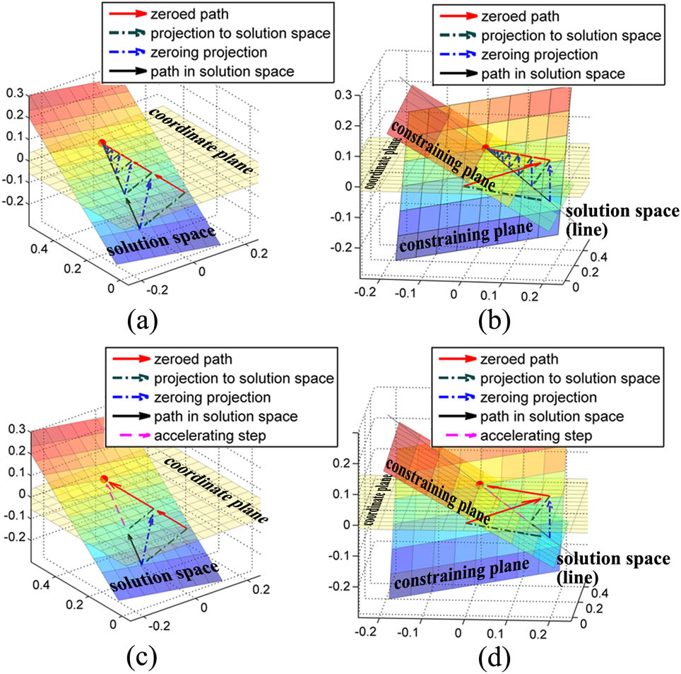
To illustrate how zeroing-Tk functions, a three-dimensional (3D) example was provided to show how the method approaches the sparse solution. The 3D example could be shown as where is the coefficient matrix and is the number of measurements; or 2 because the inverse problem of FMT is typically underdetermined. denotes the solution, whose true value is set to be sparse so that only one element is positive and the other two are zeros. denotes the measurements.
As shown in Figs. 1(a) and 1(b), if , the solution space of would be a plane and if , the solution space would be a line constrained by two planes. The systems are solved by zeroing-Tk based on an iterative Newton algorithm and an initial point .
Figure 1.Paths of 3D examples for (a) and (b) solved by zeroing-Tk and paths for (c) and (d) solved by PrSP-Tk. Red arrows: the path in the non-negative space. Dark green dashed doted arrows: the projections of the Newton algorithm projecting points into the solution space. Blue dashed dotted arrows: the zeroing steps projecting points into non-negative space from the solution space. Black arrows: the path of points in the solution space. Mauve dashed arrows: the accelerating step in the solution space.
In case of , as shown in Fig. 1(a), the red arrows denote the path in the non-negative space for the zeroing-Tk, while the black arrows denote the path of points in the solution space. The points are projected between the solution space and the coordinate plane and approach the intersection of the two planes. It illustrates how zeroing-Tk achieves sparsity. Meanwhile, it can also be seen that paths in both the coordinate plane and the solution plane are linear. In the case of , as shown in Fig. 1(b), the points are projected between the solution line and the coordinate planes and, except for the first point, both paths are also linear, which agrees with the case of . In conclusion, it could be assumed that, for the inverse problem of FMT, paths at the end of the iterations of zeroing-Tk are approximately linear.
To demonstrate the assumption, a general case is described as where is the coefficient matrix, and the system is typically underdetermined (i.e., ). denotes the distribution of the fluorescence. denotes the measurements collected on the surface of the subjects.
Zeroing-Tk can be described as the following steps: iterative Newton step projecting into in the solution space: zeroing step that is equivalent to projecting from the solution space into a hyperspace determined by a matrix , , while the hyperspace is constrained by certain coordinate planes of the n-dimensional space: .
Let the problem be simplified to , , , without losing generality. At the end of the iterations, empirically, the hyperspace determined by would be almost the same. Furthermore, assume that the initial point satisfies . Then apply the zeroing step and the Newton algorithm step, . Then the direction vector from to is . It could be derived that , where .
Let . Assume that matrix has distinct eigenvalues . Let , where denotes one of the eigenvectors corresponding to , and is a vector from the null space of . Then and it could be derived that , where denotes the point set in the solution space. If , , which means at the end of the iterations the path of points in the solution space is linear. On the other hand, if , because , after certain number of iterations the path in the solution space is approximately linear.
EED
Re-L1-NCG
L1-StOMP
IRL1
Zeroing-Tk
PrSP-Tk
3 mm
PCC
0.60
0.73
0.76
0.82
0.88
tc(s)
4.02
0.11
2.91
23.39
1.04
Ni
50
10
100
1500
44
1.5 mm
PCC
0.56
0.74
0.66
0.75
0.77
tc(s)
4.01
0.17
3.27
26.56
1.10
Ni
50
7
100
2000
50
Table 1. PCC, Computational Time (tc), and Number of Iterations (Ni) of the Homogeneous Experiments
The proposed Tikhonov-regularization-based projecting sparsity pursuit method is shown in Algorithm 1. is the regularization coefficient and usually set to [15]. is the acceleration coefficient and usually set to 0.6, which controls the acceleration projecting step size. is the slackness factor, applying slackness to the inequation that determines the acceleration projecting step size, typically set to 0.2. , typically set to be 0.1 to 1, is the sparsity error factor controlling when to stop controlling the sparsity of the solution.
It is important to study the acceleration speed of the proposed method. To simplify the problem, without regard to the intersection angle of the solution space and the non-negative space, empirically, the path is considered linear if the tangential deviations are less than 20% of the normal distance. Let , then would determine the number of iterations needed before the path could be considered linear. Because the number of iterations for the system could be considered as the maximum of the numbers determined by each eigenvalue pair and , the problem could be simplified to a problem with two eigenvalues.
Simulations were carried out to study the simplified problem. The largest eigenvalue was enumerated from 0.8 to 1 with an increment of 0.0025 and for each , the ratio was enumerated from 0 to 1 with an increment of 0.005. As shown in Fig. 2(a), for most of the enumerated eigenvalue pairs, it takes less than 100 iterations before collineation. According to Fig. 2(b), for enumerated eigenvalue pairs and , the number of iterations is the largest and about 275. Therefore, in most cases, the number of iterations before acceleration is less than 100 and it is highly relevant to of the system.
Figure 2.(a) Map of the number of iterations needed before the last path could be considered linear for different eigenvalue pairs. (b) The blue curve denotes the maximum number of iterations for given . The black curve denotes the corresponding eigenvalue for the maximum number of iterations.
To evaluate the performance of the proposed method, two sets of homogeneous-target phantom experiments and one set of heterogeneous-target phantom experiments were carried out. The experimental data were collected by a photomultiplier-tube-based time-domain FMT system previously developed in our laboratory[8]. The phantom was rotated for 360 deg, with an increment of 20 deg to obtain 18 projections for each set of the phantom experiments. In each projection, 11 detectors were uniformly placed within a detecting field of view (FOV) of 220 deg. The excitation light was at 780 nm wavelength while the collected emission light was at 840 nm. In the homogeneous-target phantom experiments, two tubes filled with 10 μM (1 M = 1 mol/L) indocyanine-green/dimethyl-sulphoxide (ICG/DMSO) were buried symmetrically inside a 3 cm diameter phantom filled with 1% intralipid. The inner diameters of the tubes were 4 mm and their outer diameters were 5 mm. The edge-edge-distances (EEDs) referring to the distance between the inner walls of the two tubes were 1.5 mm and 3 mm. In the heterogeneous-target phantom experiments, the two tubes were buried symmetrically with an EED of 4 mm, one of which was filled with 10 μM ICG/DMSO while the other was filled with 3 μM ICG/DMSO to yield half the fluorescence intensity of the former one.
The experiments were then reconstructed based on the s-EPT method combined with a restarted L1-regularized nonlinear conjugate gradient descent algorithm (re-L1-NCG)[17], an L1-norm regularization method based on stagewise orthogonal matching pursuit (L1-StOMP)[18], an iterative reweighted L1 regularization method (IRL1) that could approximate L0-norm regularization[12], zeroing-Tk, and PrSP-Tk proposed in this Letter. The forward model of s-EPT was generated through FEM, as mentioned above, and then interpolated into uniform mesh with a size of and discretization of for the reconstruction.
The parameters were adjusted to obtain as good a reconstructed image quality as possible, while keeping the crosstalk between the two targets as low as possible. In addition, the parameters of re-L1-NCG, L1-StOMP, and IRL1 were adjusted based on parameters mentioned in previous work[12,17,18]. The homogeneous-target phantom experiments were reconstructed by all five methods. In re-L1-NCG, the smooth parameter , the regularization parameter , the inner maximum iterations , and the restart iterations . In L1-StOMP, for an EED of 3 mm, the threshold parameter and the maximum number of the permissible coefficients ; for an EED of 1.5 mm, was adjusted to 0.86. In IRL1, the smoothing parameter , the maximum outer iterations , and the regularization parameters and . In zeroing-Tk, for an EED of 3 mm, the iteration and the regularization parameter ; for an EED of 1.5 mm, , and . In PrSP-Tk, for an EED of 3 mm, the acceleration coefficient , the slackness factor , the regularization parameter , and the sparsity error factor ; for an EED of 1.5 mm, was adjusted to 0.8 to eliminate the crosstalk. Meanwhile, in this Letter, the performances of IRL1 and PrSP-Tk were further evaluated in the heterogeneous-target phantom experiments. Because the performances of the other three methods are adequately demonstrated through the homogenous-target experiments, the reconstruction results of these three methods in the heterogenous-target experiments are not shown in this Letter. In IRL1, the regularization parameters were adjusted so that and for better results. In PrSP-Tk, and were adjusted to and 0.2 to obtain better quality. All the methods were implemented in MATLAB 2013 (MathWorks, Natick, MA) and all reconstructions were performed on a personal computer with Intel Core i7-6700 CPU @ 3.40 GHz and 16 Gbytes of RAM.
Except for re-L1-NCG and L1-StOMP, all the other three methods obtain a good reconstructed image quality. As can be seen in Figs. 3(a) and 4(a), in the reconstructed images of re-L1-NCG, there is severe distortion in the targets and the two targets could not be completely separated, which could also be demonstrated by the profiles shown in Figs. 3(f) and 4(f). As for L1-StOMP, the reconstructed images in Figs. 3(b) and 4(b) have an obvious distortion in the targets while the locations of the targets are inaccurate and the targets with an EED of 1.5 mm are not completely separated. For IRL1, zeroing-Tk, and the proposed PrSP-Tk, as shown in Figs. 3(c)–3(e) and 4(c)–4(e), the targets in the reconstructed images are completely separated and accurately located. In addition, PrSP-Tk avoids over-sparsity and achieves a better relative-value accuracy in the reconstruction results compared with IRL1, especially for an EED of 1.5 mm. When compared with zeroing-Tk, the proposed method is also better at accuracy, which could be illustrated by the profiles in Figs. 3(f) and 4(f) and the Pearson correlation coefficient (PCC) shown in Table 1. The PCC between the reconstruction results and the true values shows the similarity between them, and describes the reconstructed image quality in one aspect. The PCCs of IRL1 are lower than those of PrSP-Tk mainly for the sake of over-sparsity, and for an EED of 1.5 mm, the PCC of IRL1 is even lower than that of L1-StOMP. As shown in Table 1, the computational time and number of iterations of PrSP-Tk are largely reduced when compared with zeroing-Tk. In addition, the theoretically predicted numbers of iterations of the proposed method are 31 for EED of 3 mm and 36 for EED of 1.5 mm in the homogenous-target phantom experiments, which agree with the actual numbers of iterations in the reconstruction. It experimentally demonstrates the acceleration theory above. In summary, PrSP-Tk achieves the best image quality among the methods implemented, with accurate target location, accurate relative value, high spatial resolution, and good shape similarity. Furthermore, the proposed method is efficient, with the second shortest computational time that is as about one third of that of the third shortest method.
EED
Re-L1-NCG
L1-StOMP
IRL1
Zeroing-Tk
PrSP-Tk
3 mm
PCC
0.60
0.73
0.76
0.82
0.88
tc(s)
4.02
0.11
2.91
23.39
1.04
Ni
50
10
100
1500
44
1.5 mm
PCC
0.56
0.74
0.66
0.75
0.77
tc(s)
4.01
0.17
3.27
26.56
1.10
Ni
50
7
100
2000
50
Table 1. PCC, Computational Time (tc), and Number of Iterations (Ni) of the Homogeneous Experiments
Figure 3.Reconstruction results of the homogeneous experiment with an EED of 3 mm on the excitation plane by using (a) re-L1-NCG, (b) L1-StOMP, (c) IRL1, (d) zeroing-Tk, and (e) PrSP-Tk, respectively. (f) Profiles along the yellow dashed lines in (a)–(e).
Figure 4.Reconstruction results of the homogeneous experiment with an EED of 1.5 mm on the excitation plane by using (a) re-L1-NCG, (b) L1-StOMP, (c) IRL1, (d) zeroing-Tk, and (e) PrSP-Tk, respectively. (f) Profiles along the yellow dashed lines in (a)–(e).
As shown in Figs. 5(a) and 5(b), PrSP-Tk performs better and achieves good image quality for the heterogeneous-target experiments while IRL1 could not distinguish the target with lower fluorescence intensity. Because the target with lower fluorescence intensity yielded only half the fluorescence intensity of the other target, it would become more difficult to achieve good reconstructed image quality. Nevertheless, it can be seen from the profiles in Fig. 5(c) that PrSP-Tk obtains a high accuracy of the relative value and high shape similarity. However, the locations of the targets are not as accurate as in the homogeneous-target experiments, which results in a lower but acceptable PCC, as shown in Table 2. It is reasonable to surmise that it is caused by experimental noise because of the same trend in the reconstruction result of IRL1. More experiments are needed to demonstrate the underlying reason. Meanwhile, in this case, the iteration of PrSP-Tk has also been accelerated and its computational time is still shorter than that of IRL1, which agrees with the results of the homogenous-target phantom experiments.
EED
IRL1
PrSP-Tk
4 mm
PCC
0.52
0.70
Computational time (s)
4.90
0.78
Number of iterations
100
38
Table 2. PCC, Computational Time, and Number of Iterations of the Heterogeneous-Target Phantom Experiments
Figure 5.Reconstruction results of the heterogeneous experiment with an EED of 4 mm on the excitation plane by using (a) IRL1 and (b) PrSP-Tk, respectively. (c) Profiles along the yellow dashed lines in (a) and (b).
In conclusion, based on the study about the Tikhonov regularization method with zeroing strategy, the proposed Tikhonov-regularization-based projecting sparsity pursuit method reduces the iterations and computational cost, and achieves image quality not worse than that of the L1 norm or approximated L0 norm regularization methods. Moreover, the proposed method obtains a better image quality than the Tikhonov regularization method with zeroing strategy. The proposed method has a sufficiently low computational cost while obtaining the best relative value accuracy, the best location accuracy, and the best shape similarity among the methods implemented in this Letter for the homogeneous-target phantom experiments. Furthermore, the method is proved applicable for heterogeneous-target reconstruction where the approximated L0 norm method has poor performance. Good image quality, high efficiency, and wide application make the Tikhonov-regularization-based projecting sparsity pursuit method a practical method for TD-FMT reconstruction and probably for other approaches of FMT.