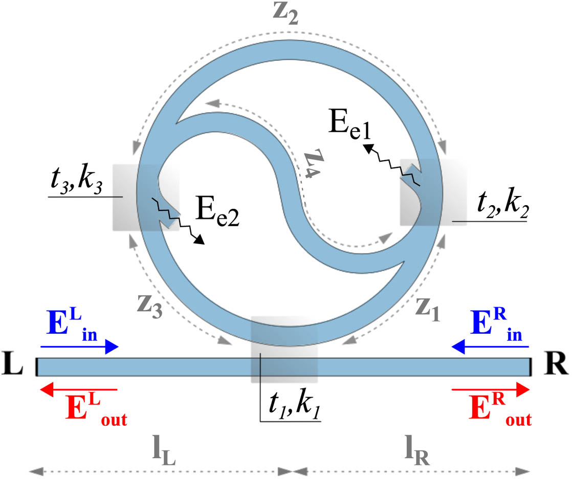
Fig. 1. Sketch of the taiji microresonator: EinL and EinR (EoutL and EoutR) are input (output) field amplitudes at the left and right facet, respectively, while Ee1 and Ee2 are the amplitudes of fields emitted as radiative dissipation; κi and ti, with i=1,2,3, are the coupling and transmission amplitudes at the different beamsplitting regions indicated by the gray squares. The gray dashed lines define the spatial size of the different segments.

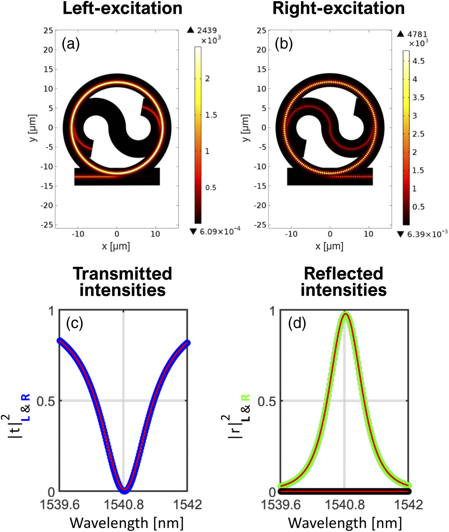
Fig. 2. Panels (a) and (b): numerical results for the field intensity in the taiji microresonator with light incident from the left and right, respectively. The geometrical dimensions are in μm. The frequency is resonant with the ring and the bus waveguide is critically coupled. The color plot shows the electric field amplitude in V/m. It is noteworthy that only light incident from the right excites the S waveguide. This highlights the non-symmetrical behavior of light reflection. Panels (c) and (d): transmitted (blue dots) and reflected intensity as a function of the incident wavelength for light incident from the left (black dots) and from the right (green dots). The red lines display the fitting results employing the analytical model.

Fig. 3. Panels (a) and (b) show the optical micrograph and the SEM image of the top and the cross-section view of a taiji microresonator, respectively. Panel (c): sketch of the experimental setup.

Fig. 4. Experimental spectra of the (a) transmitted and (b), (c) reflected intensities as a function of the incident wavelength. The blue lines show the experimental measurements while the red lines display the fitting results employing the analytical model. The bottom panels show the zoom of the transmitted (Zoom 1) and reflected (Zoom 2, 3) intensities for the resonance highlighted by the vertical dashed lines.

Fig. 5. Intensity as a function of the wavelength computed with the Eqs. (7) and (8) using the parameters of Table 1 (Appendix B) at the resonant wavelengths (λi). Precisely, the red squares are the transmitted intensity, the upward light blue triangles are the reflected intensity for light incident from right and the downward blue triangles are the reflected intensity for light incident from left. The light blue and blue dashed lines denote the average of the resonant values for the |rR(λi)|2 and the |rL(λi)|2, respectively.

Fig. 6. Map of the fields within the device, used to calculate the scattering matrix elements when light enters from the left. Labels Em, with m=1,…,6, represent complex amplitudes of the guided fields propagating in the device. Labels Ee1 and Ee2 indicate the modes that are radiated into the cladding. ti and κi, where i=1,2,3, are the transmission and coupling amplitudes at the different beamsplitting regions.

Fig. 7. Map of the fields within the device, used to calculate the scattering matrix elements when light enters from the right. Again Em, with m integers, are complex amplitudes of guided-mode fields, while Ee1 and Ee2 indicate the amplitudes of the modes that are radiated into the cladding. ti and κi, where i=1,2,3, are the transmission and coupling amplitudes at the different beamsplitting regions.

Fig. 8. Results of the simulation of the ring-bus waveguide coupling region of the taiji. Plotted curves represent the power transmission to either the bus waveguide or the ring, as a function of their mutual separation. The inset shows the distribution of electric field amplitude in the system in V/m, for a chosen distance of 335 nm. Geometrical dimensions are in μm.

Fig. 9. Results of the simulation of the ring-S-shaped waveguide coupling region of the taiji. Plotted curves represent the power transmission to either the ring or the S-shaped branch, as a function of their mutual separation. The inset shows the distribution of electric field amplitude in the system in V/m, for a chosen distance of 289 nm. Geometrical dimensions are in μm.