Optimize performance of a diffractive neural network by controlling the Fresnel number

Minjia Zheng; Lei Shi; Jian Zi

doi:10.1364/PRJ.474535

Abstract

To achieve better performance of a diffractive deep neural network, increasing its spatial complexity (neurons and layers) is commonly used. Subject to physical laws of optical diffraction, a deeper diffractive neural network (DNN) would be more difficult to implement, and the development of DNN is limited. In this work, we found controlling the Fresnel number can increase DNN’s capability of expression and its spatial complexity is even less. DNN with only one phase modulation layer was proposed and experimentally realized at 515 nm. With the optimal Fresnel number, the single-layer DNN reached a maximum accuracy of 97.08% in the handwritten digits recognition task.

1. INTRODUCTION

Supervised machine learning (ML) is widely used as one of the most essential methods for many computer vision tasks [1,2], including image classification [3,4], image segmentation [5,6], and target or saliency detection [7 –11]. Such ML algorithms require large-scale parallel computing, such as convolution operation and large matrix or vector-matrix multiplication [4,12 –15]. With the ever-increasing demand for computational resources, advances in performance of electronic devices have hit a bottleneck [16 –18]. To meet the need, a new approach called the optical neural network (ONN) has been proposed. ONN naturally provides privileges of high parallelism, high-speed calculation, and low energy consumption over electronic devices [19 –33]. ONN also has proved to be feasible and effective in solving many ML problems, and it can be used to work as a image classifier, a speech recognizer, an autoencoder, a recurrent neural network, and so on [19,20,26,27,34 –42]. Recently, an all-optical ONN framework termed diffractive deep neural network ( $D^{2} NN$ ) was proposed to provide operations of optical diffraction at the speed of light and reach hundreds of billions of connections between neurons in a power-efficient manner [26]. $D^{2} NN$ can accomplish some optical logical operations and more image processing tasks as well [42 –47].

$D^{2} NN$ regards each phase modulation pixel on the hidden layers as an artificial neuron. The connections between the hidden layers are determined by the transmission or reflection coefficient for each neuron when light is traveling forward. The values of neurons in $D^{2} NN$ are optimized by using the error backpropagation algorithm, and exact phase values $ϕ$ are converted into a relative height map h ( $h = λ ϕ / 2 π Δ n$ , where $Δ n$ is the difference of relative index between the fabricated material and the air). After $D^{2} NN$ is well trained, the passive neurons can be fabricated by 3D printing or photolithography etching [26,44,48 –50]. In the manufacturing process, the allowed phase errors are proportional to the working wavelength. This means that $D^{2} NN$ ’s performance at wavelengths shorter than infrared is below expectations. Furthermore, when hidden layers are added into $D^{2} NN$ to get better performance, the accumulation of errors owing to the misalignment of multiple layers also remains a big problem. With the growing needs of spatial complexity, especially neurons and layers, implementation difficulties arise as well. Hence, reducing $D^{2} NN$ ’s space complexity deserves further study while its capability of expression is kept.

In this work, we introduce a new approach toward designing the phase-only all-optical ML framework by controlling the Fresnel number that describes the regime of diffraction effects. Making this diffraction-related parameter wet-set will optimize the performance of a diffractive neural network (DNN) instead of increasing the hidden layers in $D^{2} NN$ . To demonstrate how the Fresnel number works, we propose the framework of a single-layer diffractive neural network (SL-DNN), since its space complexity is minimized to a great extent. We find that DNN with even single phase modulation layer can provide good capability of expression. In numerical experiments, we achieved a blind testing accuracy of 97.08% in the Mixed National Institute of Standards and Technology (MNIST) handwritten digit recognition task [51]. In our experiments, we implemented SL-DNN, tested 1000 samples, and achieved an accuracy rate of 92.70%.

Sign up for Photonics Research TOC. Get the latest issue of Photonics Research delivered right to you！Sign up now

2. THEORETICAL ANALYSIS

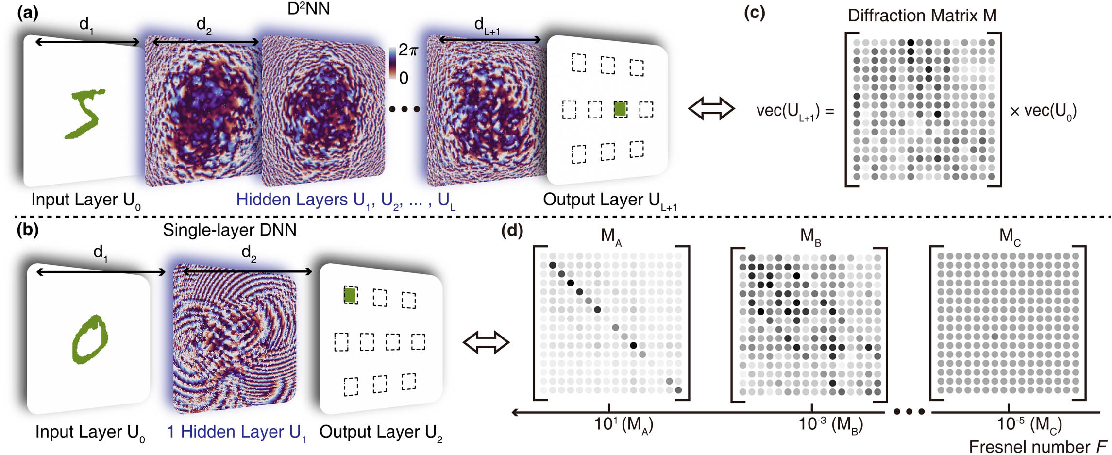
Phase-only $D^{2} NN$ describes a multidiffraction process to arbitrarily modulate the wavefront of light diffracted from an input plane. The process can be treated as a matrix multiplication operation on the input plane without the nonlinear activation layer. As illustrated in Figs. 1(a) and 1(c), the diffraction process of multilayer diffraction can be simply represented by a complex-valued matrix $M$ , and the optical intensity after the entire diffraction process can be expressed as $o = {| u_{L + 1} |}^{2} = {| M u_{0} |}^{2},$ (1)where $u_{0}$ and $u_{L + 1}$ are the vectorized optical field at the input and output layer, and $o$ is the optical intensity of the output layer. In Eq. (1), $L$ represents the number of phase modulation layers. The diffraction process between the successive two layers can be characterized as $u_{i + 1}^{input} = D u_{i}^{output},$ (2)where $u_{i + 1}^{input}$ is the optical field before layer $i + 1$ and $u_{i}^{output}$ is the optical field after layer $i$ , and $D$ is the diffraction process between the two successive layers and is a complex-valued symmetric matrix. The phase modulation layer $p_{i}$ is added after $u_{i + 1}^{input}$ , and the optical field becomes $u_{i + 1}^{output} = u_{i + 1}^{input} \circ p_{i} .$ (3)“ $\circ$ ” represents the Hadamard product, and the operation can be transformed to matrix multiplication. Therefore, Eq. (3) can be rewritten as $u_{i + 1}^{output} = diag (p_{i}) D u_{i}^{output} .$ (4)So far, the diffraction matrix $M$ can be described by $M = D \prod_{i = L}^{1} [diag (p_{i}) D] .$ (5)

$Schematic diagram of the frameworks of (a) deep and (b) SL-DNN; (c) the entire diffraction and multi-layer phase modulation process can be regarded as a matrix multiplication by diffraction matrix M. (d) The diffraction matrix of SL-DNN with different values of Fresnel number can be represented by MA (∼101), MB (∼10−3), and MC (∼10−5).$

Figure 1.Schematic diagram of the frameworks of (a) deep and (b) SL-DNN; (c) the entire diffraction and multi-layer phase modulation process can be regarded as a matrix multiplication by diffraction matrix $M$ . (d) The diffraction matrix of SL-DNN with different values of Fresnel number can be represented by $M_{A}$ ( $\sim 10^{1}$ ), $M_{B}$ ( $\sim 10^{- 3}$ ), and $M_{C}$ ( $\sim 10^{- 5}$ ).

In other words, $M$ , as well as $D^{2} NN$ , is the transformation matrix that maps vectors of the input plane ( $u_{0}$ ) into the output plane ( $u_{L + 1}$ ) in an $N^{2}$ -dimensional Hilbert space, where $N$ is the pixel number of every layer’s side length. $M$ should have two major properties to finish the classification task. One is that the row vectors of $M$ need to be incompletely orthogonal, which allows $M$ to implement many-to-one mapping so that $D^{2} NN$ has the ability to cluster inputs of the same class. The other is that the value of rows of $M$ has to be arbitrary. It provides the ability to separate the different kinds of samples. To satisfy these two requirements, research has focused on increasing neurons and layers of $D^{2} NN$ , in other words, increasing its spatial complexity. In Fig. 1(c), the diffraction matrix $M$ of multilayer $D^{2} NN$ provides both the many-to-one mapping and the arbitrariness. Generally speaking, $D^{2} NN$ ’s classification ability is strengthened when the number of layers is increased [26]. With the increase of neurons and layers, the difficulty of preparing phase modulation neurons and the layer-to-layer alignment increases.

It is commonly considered that $D^{2} NN$ with few layers can provide only one of these requirements mentioned above. In Figs. 1(b) and 1(d), the diffraction matrix $M$ of DNN with one hidden layer can be divided by the Fresnel number $F$ into three cases, where $F = \frac{a^{2}}{λ d},$ (6)and $a$ is the pixel area, $λ$ is the working wavelength, and $d$ is the layer-to-layer distance. As shown in Fig. 1(d), when $F$ is approximately $10^{1}$ , it also means in the case of very near diffraction, the row vectors of $M_{A}$ are arbitrary but completely orthogonal. It means only elements on the diagonal of the diffraction matrix have the capability to modulate the incident light. The input and the output layers are mapped one-to-one by $M_{A}$ , and it cannot afford the requirement of many-to-one mapping. Likewise, when $F$ is a pretty small value (approximately $10^{- 5}$ ), it also means in the case of very far diffraction, all row vectors of $M_{C}$ are almost linearly related. In $M_{C}$ , all elements are almost identical, which means $rank (M_{C}) \approx 1 ≪ rank (M_{C} | u_{0})$ . All $u_{0}$ will have the same pattern at the output layer, and DNN offers no ability to modulate the incoming light. This leads to the result that the diffraction matrix can only provide many-to-one mapping but cannot separate samples from different classes.

In order to resolve the contradiction between DNN’s preparation difficulty and the requirements of its ability of expression, we propose a new approach for regulating an SL-DNN by controlling the Fresnel number $F$ so that it can also meet both requirements mentioned above. DNN regards connections originating from each neuron as the kernels of convolutional neural network. If $F$ is too large, the kernel size will be $1 \times 1$ , and if $F$ is too small, the kernel size will be very large and the values of the kernel are almost identical. An appropriate $F$ provides both enough receptive field and different values of the kernel. In Fig. 1(d), $M_{B}$ with a proper $F$ is more like the $M$ in Fig. 1(c) than $M_{A}$ and $M_{C}$ . $F$ determines the property of $M$ .

We can compare $M$ with $M_{B}$ and find out that an appropriate $F$ can provide a many-to-one mapping of the input layer to the output layer even if only one phase modulation layer is applied. In the meantime, good arbitrariness can support SL-DNN to accomplish tasks like MNIST handwritten digit recognition. Furthermore, when $F \in (4 / N^{2},2 / N)$ , SL-DNN can provide enough ability of expression and show good performance in such a classification job. More information is provided in Appendix A.

3. IMPLEMENTATION OF DNN AT DIFFERENT FRESNEL NUMBERS

A. Training Methods

In Fig. 2, SL-DNN consists of two diffraction and one phase modulation process. The first diffraction is from input layer to the phase modulation layer (hidden layer), and the second diffraction is from the hidden layer to the output layer. Note that $F$ is given by the pixel size $a$ , the diffraction distance $d$ , and the working wavelength $λ$ . To get different $F$ in the experiment, there is no need to change $a$ or $d$ every time. We can simply resize the input layer, and this operation equivalently changes $F$ when the parameters of DNN are fixed. We use the angular spectrum (AS) method to simulate these two diffraction processes. This can be written as $F (u_{i + 1}) = F (u_{i}) \circ H,$ (7)where $u_{i}$ and $u_{i + 1}$ are the optical field at layer $i$ and $i + 1$ , $H$ is the transfer function in the AS method, and $F (\cdot)$ is the Fourier transform. The process of phase modulation is provided by a Hadamard product of the incoming optical field and the phase delay part. Phase values are optimized via the error backpropagation algorithm. We use softmax-cross-entropy (SCE) loss and the mean squared error (MSE) loss as loss functions for our training. SCE loss can be defined as $e_{SCE} = - \sum_{j = 1}^{T} y_{j} \log s_{j},$ (8)and $T$ represents the number of categories, $y_{j}$ is the one-hot encoding of ground truth, and $s_{j} = e^{o_{j}} / Σ_{i = 1}^{T} e^{o_{i}}$ is the softmax operation of output, where $o_{i}$ is the sum of light intensity in the selected region of digit $i$ on the output layer shown in Fig. 2. MSE loss can be defined as $e_{MSE} = ∥ o - o_{gt} ∥_{2}^{2},$ (9)where $o$ is the light intensity on the output plane and $o_{gt}$ is the ground truth.

$Schematic experimental setup of SL-DNN. A laser beam at 515 nm was used. The linearly polarized beam was incident on the DMD and images of digits in the MNIST data set were illuminated by DMD. After that, light was normally reflected and propagated to the SLM. SLM modulates the phase of light field and it was reflected by a beam splitter (BS). The output layer is shown by the incoming light received by a CMOS camera. The image dimensions of digits are resized to N and Nr to show different F when the diffraction distance d is fixed. Colors of two light paths are only to distinguish between two SL-DNNs with different F.$

Figure 2.Schematic experimental setup of SL-DNN. A laser beam at 515 nm was used. The linearly polarized beam was incident on the DMD and images of digits in the MNIST data set were illuminated by DMD. After that, light was normally reflected and propagated to the SLM. SLM modulates the phase of light field and it was reflected by a beam splitter (BS). The output layer is shown by the incoming light received by a CMOS camera. The image dimensions of digits are resized to $N$ and $N_{r}$ to show different $F$ when the diffraction distance $d$ is fixed. Colors of two light paths are only to distinguish between two SL-DNNs with different $F$ .

B. Simulation Results

To demonstrate the performance of SL-DNN in the MNIST handwritten classification task, we trained the network with 60,000 images of 10 digits. After SL-DNN had been well trained, we numerically tested the model with a test set of another 10,000 images. In Fig. 3(b), SL-DNN achieves an accuracy of 94.94% in blindly testing its performance when we use SCE and MSE loss functions whose ratio is 0.2:0.8. We set the dimension of every layer to be $200 \times 200$ and selected an appropriate $F$ to achieve SL-DNN’s best performance. SL-DNN also achieves the highest accuracy of 97.08% when using SCE loss only. More information about the simulation and experiments is provided in Appendix A.

Figure 3.(a) Images of MNIST handwritten input digits are binarized. Ten light intensity detector regions $I_{0}, I_{1}, \dots, I_{9}$ are set on the output plane, respectively. The detector with maximum sum of intensity shows the predicted number. (b) The confusion matrix and energy distribution percentage of $F$ show numerical test results of blindly testing 10,000 images, and it achieves the max accuracy rate of 94.94%. (c) The confusion matrix and energy distribution percentage for the experimental results. We use 1000 different handwritten digits in the test set as input and achieve an accuracy rate of 92.70%.

C. Experimental Results

To implement SL-DNN, we adapted the experimental setup shown in Fig. 2. In the experiment, we used a programmable digital micromirror device (DMD) to form the input patterns of data sets and another programmable reflective phase-only liquid-crystal spatial light modulator (LC-SLM) as the phase modulation layer. We also used a complementary metal oxide semiconductor (CMOS) image sensor to read the light intensity at the output layer. The working wavelength of light was at 515 nm based on a diode-pumped laser. In our experiment, input digits were illuminated by the collimated laser beam incident onto the DMD, and then images in the test set were displayed on DMD. Before that, images were resized and binarized. We used a 2-bit reflective DMD to form the shapes of different input digits. After the light was reflected and traveled a distance of $d_{1}$ ( $\approx 164.7 mm$ ), we used a reflective phase-only SLM as the phase modulation layer. This will lead to a problem: the reflected light coming from the untrained pixels outside the region we have trained will also affect the optical field distribution at output plane. So, we enlarge the dimension of phase modulation layer to $800 \times 800$ to avoid this problem. We trained SL-DNN, and phase values of the hidden layer are uploaded to the SLM. After the second diffraction of distance of $d_{2}$ ( $\approx 173.5 mm$ ), a CMOS camera received the light intensity signal. As shown in Fig. 3(a), we manually selected the ten regions of output light distribution captured by the CMOS camera. Of these ten regions, the highest total light intensity shows the recognized digit. In Fig. 3(c), we got an accuracy rate of 92.70% in blindly testing 1000 randomly selected samples in the test set when $N = 200$ . In Fig. 3, we also provide the energy distribution of the ten selected regions. It is obvious that light has been focused in the specific region of each test sample. Note that, when we get into the experiment, errors in the diffraction distance measurement and of the instruments themselves cause little energy misdistribution on the output layer in comparison to simulation results. The fill factors of the DMD and SLM also slightly affect the reconstruction of the diffraction process. All these lead to a decrease in accuracy of the experiments compared with numerical simulation.

To illustrate the relation between Fresnel number $F$ and the performance of SL-DNN further, we tested the network at different $F$ numerically and experimentally. The experimental setup is fixed so that we can see from Fig. 2 that resizing the input images equivalently changes the $F$ . We can see from Fig. 4 that at different wavelengths of light, there is the same $F$ range, which is from approximately $10^{- 4}$ to $10^{- 2}$ . If $F$ is in this range, SL-DNN can provide good performance and has good ability of expression. We also experimentally tested SL-DNN at different $F$ by resizing the input images on DMD from initially $200 \times 200$ to $50 \times 50$ , $500 \times 500$ , and $800 \times 800$ , respectively, while keeping the experiment setup fixed. The accuracy of another three experiments we have gotten is 64.10%, 86.60%, and 74.10%, respectively. More information about the experiment is shown in Appendix B.

Figure 4.Accuracy of SL-DNN as an MNIST handwritten digit classifier with changing Fresnel number $F$ . For different working wavelengths, SL-DNN has a same range of $F$ approximately from $10^{- 4}$ to $10^{- 2}$ , which shows SL-DNN’s good performance.

4. CONCLUSION AND DISCUSSION

A. Conclusion

To conclude, we propose a new approach that shows that controlling the diffraction-related parameter $F$ can improve the network’s capability of expression and optimize the performance of the DNN. As long as the diffractive parameters are well set, a DNN with only single phase-only modulation layer can also be applied to accomplish object classification tasks. As the space complexity is reduced, it is possible to implement DNN at a shorter wavelength. We numerically tested SL-DNN performance in MNIST handwritten recognition task and reached the highest accuracy rate of 97.08%. We then experimentally realized SL-DNN in the visible range by using a DMD as the input layer and a reflective phase-only SLM as the phase modulation layer. We also experimentally tested the performance of SL-DNN and got an accuracy rate of 92.70%. This article reveals a new modulation dimension to optimize the performance of DNN and makes it possible to implement more complex and miniaturized all ONN devices.

B. Discussion on the Difference between the Fresnel Number Model and Fully Connected Model

The fully connected model proposed by Lin et al. [26] and Chen et al. [48] ensures that pixels on the successive phase modulation layers are actually linked. It shows that the diffraction distance should be bounded below by $d_{\min}$ . Their conclusion is appropriate for multilayer DNNs. In this article, we show that if diffraction distance is substituted for the Fresnel number, it should be bounded above by $F_{\max}$ . This conclusion is self-consistent with Lin’s and Chen’s work. Moreover, we find that the Fresnel number is also bounded below by $F_{\min}$ , and it is merely related to the dimension of inputs. When the Fresnel number is in this optimal range, which has both upper and lower bounds, DNN can have a good performance. Our conclusion further applies to DNN with a single-phase modulation layer. More information is shown in Appendix A.

C. Discussion on DNN at Broadband Incoherent Light Incidence

To make DNN into a practical application, the optimization of DNN in the case of broadband incoherent light incidence is worth investigation. Speaking of broadband illumination, we first think of multichannel DNN with coherent light. SLMs can be used as gratings to separate different colors of light and as lenses to focus light at different locations. For the single frequency of light, the theory on the performance of network with respect to the Fresnel number still works. When the answers from the DNN from every channel are combined or retrieved, broadband DNNs can be realized. Since there are difficulties in the implementation of such a DNN with a single SLM, more SLMs and metasurfaces can be used to respond to light at different frequencies.

Moreover, holography techniques are useful in the implementation of DNNs. Self-interference incoherent digital holography (SIDH) is one of the techniques that can record the holographic information from the object illuminated by the incoherent light [52]. We believe that overlay phase values of SLMs can be trained to realize classification tasks, since the initial phase encoding can be optimized by the Gerchberg–Saxton algorithm [53].

D. Discussion on Optical Nonlinearity of DNN

Optical nonlinearity can be implemented by using nonlinear materials as diffractive layers in DNNs. In the framework of DNNs, the only nonlinear operation without optical nonlinearity is the recording of light intensity at the camera. This kind of operation is different from the commonly known “nonlinear activation function.” The difference is that it has no “activation” judgment. When we add a complex-valued activation function, such as modReLU, after the phase modulation layer, the performance of the DNN will be improved. More information is shown in Appendix A. Although nonlinear activation function is applied, SL-DNN cannot be called a “deep” neural network. When activation functions or optical nonlinearity layers are applied after every layer in multilayer DNNs, a deep nonlinear DNN can be realized and will have better performance. Optical nonlinearity requires immense light intensity, so that the implementation of nonlinear DNN at low-light intensity deserves further investigation.

APPENDIX A: NUMERICAL EXPERIMENTS

1.Data Set Preprocessing

0,1, \dots,9

2.Derivation of Optimal Range of the Fresnel Number

d

I (x, y) = I_{0} {sinc}^{2} (α) {sinc}^{2} (β),

F

Figure 5.Optical intensity of single-pixel illumination at different F.

Figure 6.Classification accuracy, MSE, and SCE loss of SL-DNN trained with MSE and SCE loss function for MNIST handwritten recognition.

Figure 7.Accuracy of SL-DNN in MNIST handwritten recognition within a certain range of phase error.

$Accuracy of SL-DNN in MNIST handwritten recognition within a certain range of diffraction distance error.$

Figure 8.Accuracy of SL-DNN in MNIST handwritten recognition within a certain range of diffraction distance error.

Figure 9.Confusion matrix and energy distribution of SL-DNN at MNIST recognition task using SCE loss function only.

Figure 10.Confusion matrix and energy distribution of SL-DNN at fashion MNIST recognition task.

Figure 11.Confusion matrix and energy distribution of SL-DNN with modReLU nonlinear activation function at MNIST and fashion MNIST recognition task.

APPENDIX B: EXPERIMENTS

1.Experimental Setup

The experimental setup of the SL-DNN is shown in Fig. 12. A linear polarizer (LP) was placed to get linearly polarized light. Another LP filter was placed before the CMOS image sensor, and it was used as an analyzer whose direction of polarization was oriented parallel to the long axis of the SLM. A half-wave (HW) plate was placed between the LP and the DMD to eliminate zero-order diffraction as much as possible. The angle between incident light and its normal is about 24°.

Figure 12.Experimental setup of SL-DNN.

Figure 13.Phase values modulated by SLM without calibration (red line) and the desired shifted phase (green line).

Figure 14.Experiment results of resizing the images of input digits to 50, 500, and 800, respectively, and equivalent Fresnel number $F$ is approximately $1 \times 10^{- 2}$ , $8 \times 10^{- 4}$ , and $5 \times 10^{- 5}$ .

References

[1] R. Szeliski. Computer Vision: Algorithms and Applications(2010).

[2] Y. LeCun, Y. Bengio, G. Hinton. Deep learning. Nature, 521, 436-444(2015).

[3] P. Bartlett, A. Krizhevsky, F. Pereira, I. Sutskever, C. Burges, G. E. Hinton, L. Bottou, K. Weinberger. Advances in Neural Information Processing Systems 25 (NIPS 2012): 26th Annual Conference on Neural Information Processing Systems 2012(2012).

[4] D. Touretzky, Y. LeCun, B. Boser, J. Denker, D. Henderson, R. Howard, W. Hubbard, L. Jackel. Advances in Neural Information Processing Systems, 2(1989).

[5] R. M. Haralick, L. G. Shapiro. Image segmentation techniques. Comput. Vis. Graph. Image Process., 29, 100-132(1985).

[6] S. Minaee, Y. Y. Boykov, F. Porikli, A. J. Plaza, N. Kehtarnavaz, D. Terzopoulos. Image segmentation using deep learning: a survey. IEEE Trans. Pattern Anal. Mach. Intell., 44, 3523-3542(2021).

[7] A. Borji, M.-M. Cheng, H. Jiang, J. Li. Salient object detection: A benchmark. IEEE Trans. Image Process., 24, 5706-5722(2015).

[8] H. Fu, X. Cao, Z. Tu. Cluster-based co-saliency detection. IEEE Trans. Image Process., 22, 3766-3778(2013).

[9] W. Wang, J. Shen, L. Shao. Video salient object detection via fully convolutional networks. IEEE Trans. Image Process., 27, 38-49(2017).

[10] A. Wang, M. Wang. RGB-D salient object detection via minimum barrier distance transform and saliency fusion. IEEE Signal Process. Lett., 24, 663-667(2017).

[11] A. Chaurasia, E. Culurciello. LinkNet: exploiting encoder representations for efficient semantic segmentation. IEEE Visual Communications and Image Processing (VCIP), 1-4(2017).

[12] O. Russakovsky, J. Deng, H. Su, J. Krause, S. Satheesh, S. Ma, Z. Huang, A. Karpathy, A. Khosla, M. Bernstein, A. C. Berg, F.-F. Li. Imagenet large scale visual recognition challenge. Int. J. Comput. Vis., 115, 211-252(2015).

[13] W. Zhang, K. Itoh, J. Tanida, Y. Ichioka. Parallel distributed processing model with local space-invariant interconnections and its optical architecture. Appl. Opt., 29, 4790-4797(1990).

[14] W. S. Sarle. Neural networks and statistical models. Proceedings of the 19th Annual SAS Users Group International Conference(1994).

[15] R. Hamerly, L. Bernstein, A. Sludds, M. Soljačić, D. Englund. Large-scale optical neural networks based on photoelectric multiplication. Phys. Rev. X, 9, 021032(2019).

[16] A. Adamatzky. Unconventional Computing: A Volume in the Encyclopedia of Complexity and Systems Science(2018).

[17] J. M. Shainline, S. M. Buckley, R. P. Mirin, S. W. Nam. Superconducting optoelectronic circuits for neuromorphic computing. Phys. Rev. Appl., 7, 034013(2017).

[18] H. N. Khan, D. A. Hounshell, E. R. Fuchs. Science and research policy at the end of Moore’s law. Nat. Electron., 1, 14-21(2018).

[19] J. Bueno, S. Maktoobi, L. Froehly, I. Fischer, M. Jacquot, L. Larger, D. Brunner. Reinforcement learning in a large-scale photonic recurrent neural network. Optica, 5, 756-760(2018).

[20] T. W. Hughes, M. Minkov, Y. Shi, S. Fan. Training of photonic neural networks through in situ backpropagation and gradient measurement. Optica, 5, 864-871(2018).

[21] P. R. Prucnal, B. J. Shastri, M. C. Teich. Neuromorphic Photonics(2017).

[22] D. Pérez, I. Gasulla, P. D. Mahapatra, J. Capmany. Principles, fundamentals, and applications of programmable integrated photonics. Adv. Opt. Photon., 12, 709-786(2020).

[23] X. Xu, M. Tan, B. Corcoran, J. Wu, A. Boes, T. G. Nguyen, S. T. Chu, B. E. Little, D. G. Hicks, R. Morandotti, A. Mitchell, D. J. Moss. 11 tops photonic convolutional accelerator for optical neural networks. Nature, 589, 44-51(2021).

[24] B. J. Shastri, A. N. Tait, T. Ferreira de Lima, W. H. Pernice, H. Bhaskaran, C. D. Wright, P. R. Prucnal. Photonics for artificial intelligence and neuromorphic computing. Nat. Photonics, 15, 102-114(2021).

[25] J. Feldmann, N. Youngblood, M. Karpov, H. Gehring, X. Li, M. Stappers, M. Le Gallo, X. Fu, A. Lukashchuk, A. S. Raja, J. Liu, C. D. Wright, A. Sebastian, T. J. Kippenberg, W. H. P. Pernice, H. Bhaskaran. Parallel convolutional processing using an integrated photonic tensor core. Nature, 589, 52-58(2021).

[26] X. Lin, Y. Rivenson, N. T. Yardimci, M. Veli, Y. Luo, M. Jarrahi, A. Ozcan. All-optical machine learning using diffractive deep neural networks. Science, 361, 1004-1008(2018).

[27] Y. Shen, N. C. Harris, S. Skirlo, M. Prabhu, T. Baehr-Jones, M. Hochberg, X. Sun, S. Zhao, H. Larochelle, D. Englund, M. Soljačić. Deep learning with coherent nanophotonic circuits. Nat. Photonics, 11, 441-446(2017).

[28] A. N. Tait, T. F. De Lima, E. Zhou, A. X. Wu, M. A. Nahmias, B. J. Shastri, P. R. Prucnal. Neuromorphic photonic networks using silicon photonic weight banks. Sci. Rep., 7, 7430(2017).

[29] M. Hermans, M. Burm, T. Van Vaerenbergh, J. Dambre, P. Bienstman. Trainable hardware for dynamical computing using error backpropagation through physical media. Nat. Commun., 6, 6729(2015).

[30] D. Brunner, M. C. Soriano, C. R. Mirasso, I. Fischer. Parallel photonic information processing at gigabyte per second data rates using transient states. Nat. Commun., 4, 1364(2013).

[31] M. M. P. Fard, I. A. D. Williamson, M. Edwards, K. Liu, S. Pai, B. Bartlett, M. Minkov, T. W. Hughes, S. Fan, T.-A. Nguyen. Experimental realization of arbitrary activation functions for optical neural networks. Opt. Express, 28, 12138-12148(2020).

[32] S. Pai, Z. Sun, T. W. Hughes, T. Park, B. Bartlett, I. A. D. Williamson, M. Minkov, M. Milanizadeh, N. Abebe, F. Morichetti, A. Melloni, S. Fan, O. Solgaard, D. A. B. Miller. Experimentally realized in situ backpropagation for deep learning in nanophotonic neural networks(2022).

[33] G. Wetzstein, A. Ozcan, S. Gigan, S. Fan, D. Englund, M. Soljačić, C. Denz, D. A. Miller, D. Psaltis. Inference in artificial intelligence with deep optics and photonics. Nature, 588, 39-47(2020).

[34] I. Chakraborty, G. Saha, A. Sengupta, K. Roy. Toward fast neural computing using all-photonic phase change spiking neurons. Sci. Rep., 8, 12980(2018).

[35] J. Chang, V. Sitzmann, X. Dun, W. Heidrich, G. Wetzstein. Hybrid optical-electronic convolutional neural networks with optimized diffractive optics for image classification. Sci. Rep., 8, 12324(2018).

[36] L. Mennel, J. Symonowicz, S. Wachter, D. K. Polyushkin, A. J. Molina-Mendoza, T. Mueller. Ultrafast machine vision with 2D material neural network image sensors. Nature, 579, 62-66(2020).

[37] Y. Zuo, B. Li, Y. Zhao, Y. Jiang, Y.-C. Chen, P. Chen, G.-B. Jo, J. Liu, S. Du. All-optical neural network with nonlinear activation functions. Optica, 6, 1132-1137(2019).

[38] X. Luo, Y. Hu, X. Ou, X. Li, J. Lai, N. Liu, X. Cheng, A. Pan, H. Duan. Metasurface-enabled on-chip multiplexed diffractive neural networks in the visible. Light Sci. Appl., 11, 158(2022).

[39] J. Li, Y.-C. Hung, O. Kulce, D. Mengu, A. Ozcan. Polarization multiplexed diffractive computing: all-optical implementation of a group of linear transformations through a polarization-encoded diffractive network. Light Sci. Appl., 11, 153(2022).

[40] F. Ashtiani, A. J. Geers, F. Aflatouni. An on-chip photonic deep neural network for image classification. Nature, 606, 501-506(2022).

[41] T. W. Hughes, I. A. Williamson, M. Minkov, S. Fan. Wave physics as an analog recurrent neural network. Sci. Adv., 5, eaay6946(2019).

[42] H. Dou, Y. Deng, T. Yan, H. Wu, X. Lin, Q. Dai. Residual D²NM: training diffractive deep neural networks via learnable light shortcuts. Opt. Lett., 45, 2688-2691(2020).

[43] C. Qian, X. Lin, X. Lin, J. Xu, Y. Sun, E. Li, B. Zhang, H. Chen. Performing optical logic operations by a diffractive neural network. Light Sci. Appl., 9, 59(2020).

[44] S. Jiao, J. Feng, Y. Gao, T. Lei, Z. Xie, X. Yuan. Optical machine learning with incoherent light and a single-pixel detector. Opt. Lett., 44, 5186-5189(2019).

[45] Z. Wu, M. Zhou, E. Khoram, B. Liu, Z. Yu. Neuromorphic metasurface. Photon. Res., 8, 46-50(2020).

[46] Z. Wu, Z. Yu. Small object recognition with trainable lens. APL Photon., 6, 071301(2021).

[47] T. Zhou, X. Lin, J. Wu, Y. Chen, H. Xie, Y. Li, J. Fan, H. Wu, L. Fang, Q. Dai. Large-scale neuromorphic optoelectronic computing with a reconfigurable diffractive processing unit. Nat. Photonics, 15, 367-373(2021).

[48] H. Chen, J. Feng, M. Jiang, Y. Wang, J. Lin, J. Tan, P. Jin. Diffractive deep neural networks at visible wavelengths. Engineering, 7, 1483-1491(2021).

[49] Y. Hu, X. Luo, Y. Chen, Q. Liu, X. Li, Y. Wang, N. Liu, H. Duan. 3D-integrated metasurfaces for full-colour holography. Light Sci. Appl., 8, 86(2019).

[50] Y. Chen, Z. Shu, S. Zhang, P. Zeng, H. Liang, M. Zheng, H. Duan. Sub-10 nm fabrication: methods and applications. Int. J. Extreme Manuf., 3, 032002(2021).

[51] Y. LeCun, L. Bottou, Y. Bengio, P. Haffner. Gradient-based learning applied to document recognition. Proc. IEEE, 86, 2278-2324(1998).

[52] A. W. Lohmann. Wavefront reconstruction for incoherent objects. J. Opt. Soc. Am., 55, 1555-1556(1965).

[53] R. W. Gerchberg, W. O. Saxton. A practical algorithm for the determination of plane from image and diffraction pictures. Optik, 35, 237-246(1972).