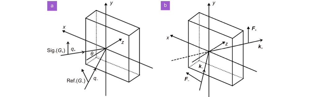
Fig. 1. Schematic of polarization holography: (a) recording process; (b) reconstruction process.

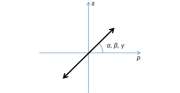
Fig. 2. The definition of the orientation of the polarized wave under two orthogonal basic unit vectors p and s coordination.

Fig. 3. The definition of basic unit p vectors in the process of (a) recording and (b) reconstruction.

Fig. 4. The relationship between NDE and the polarization angle of reading wave. The double arrow symbol represents the polarization angle of reading wave. Figure reproduced with permission from ref.³², The Optical Society.

Fig. 5. The variation of NDE and polarization angle of the reconstructed wave with the polarization angle of reading wave under different recording conditions. The polarization angles of the signal wave are: 0°, 45° and 90°, respectively. (a) The variation of NDE of reconstructed wave. The theoretical value is cos²γ curve. (b) The variation of polarization angle of the reconstructed wave. Figure reproduced with permission from ref.²⁹, Chinese Laser Press.

Fig. 6. The simulated value of reconstructed wave changes with the polarization angle of reading wave under different recording conditions. All the polarization angles of the reference wave are p-polarized. (a) The variation of polarization angle of the reconstructed wave. (b) The variation of NDE of the reconstructed wave.

Fig. 7. The variation of polarization angle of the reconstructed wave with the polarization angle of reference and reading waves. Figure reproduced with permission from ref. ³¹, The Optical Society.

Fig. 8. The variation of the s- and p-polarized components in the reconstructed wave with the HWP2 angle under different interference angles.The interference angles are 15.8°, 26.2°, 38.1° and 58.5°, respectively, which are distinguished by lines of different colors. The polarization angle of the reading wave is twice the fast-axis angle of HWP2. Figure reproduced with permission from ref. ³⁴, Chinese Laser Press.

Fig. 9. Optical setup of linear polarization holography. SF, spatial filter; PBS, polarization beam splitter; SH, shutters; HWP, half-wave plates. Figure reproduced with permission from ref.¹⁹, The Optical Society.

Fig. 10. The variation of the s- and p-polarized components in the reconstructed wave with the HWP1 angle. Figure reproduced with permission from ref.¹⁹, The Optical Society.

Fig. 11. Optical setup for four-channel polarization holographic recording. SF, spatial filter; PBS, polarization beam splits; SH, shutters; HWP, half-wave plates; BS, beam splitter; SLM, spatial light modulator. Figure reproduced with permission from ref.³², The Optical Society.

Fig. 12. Images reconstructed in four-channel holographic image recording. (a–d) Original transmitted images before holographic recording. (e) and (f) reconstructed image of the p-polarized reading wave. (g) and (h) reconstructed image of the s-polarized reading wave. Figure reproduced with permission from ref.³², The Optical Society.

Fig. 13. Schematic of experiment.PBS, polarization beam splitter; M, mirror; P, polarizer; HWP, half wave plate; L, lens. Figure reproduced with permission from ref.³³, The Optical Society.

Fig. 14. The intensity and polarization distributions of the vector beams with azimuthal index of m=2, θ₀=30°. (a–e) The simulation of reconstructed wave intensity distribution after changing the transmission axis of polarizer (30°, 120°, 150°, 180°). (f–j) The corresponding experimental results. Figure reproduced with permission from ref.³³, The Optical Society.

Fig. 15. Experimental results.(a) Signal wave is s-polarized. (b) Signal wave is p-polarized. (c) Signal wave is 45°-polarized. All reference and reading waves are s-polarized. Notice that the vertical scale in different graphs is different. Figure reproduced with permission from ref.²¹, The Springer Nature.

Fig. 16. Simulated variation of NDE of reconstructed wave with polarization angle of reading wave. (a) The variation of the s- and p-polarized components in the reconstructed wave with polarization angle of reading wave. (b) The variation of the polarization angle of reconstructed wave with polarization angle of reading wave.

Fig. 17. Simulated variation of NDE of reconstructed wave with polarization angle of reading wave. (a) The variation of the s- and p-polarized components in the reconstructed wave with polarization angle of reading wave. (b) The variation of the polarization angle of reconstructed wave with polarization angle of reading wave.

Fig. 18. Simulated variation of NDE of reconstructed wave with polarization angle of reading wave. (a) The variation of the s- and p-polarized components in the reconstructed wave with polarization angle of reading wave. (b) The variation of the polarization angle of reconstructed wave with polarization angle of reading wave.

Fig. 19. The variation of reconstructed wave with exposure energy under different recording conditions. (a) The variation of polarization angle of reconstructed wave with exposure energy, where polarization angles of signal wave are 0°, 15°, 30°, 45°, 60°, 75°, and 90°. (b) The variation of exposure response coefficient A/B with exposure energy for different linearly polarized signal wave, where polarization angles of signal wave are 15°, 30°, 45°, 60°, 75°. Figure reproduced with permission from ref.²⁷, The Optical Society.

Fig. 20. The variation of diffraction efficiency with exposure energy.Figure reproduced with permission from ref.²⁷, The Optical Society.

Table 0. Dual-channel polarization multiplexing experiment scheme using FRE or ORE.

Table 0. FRE and ORE independent of exposure energy under general conditions.

Table 0. Reconstruction characteristics of linear polarization holography under the balanced condition of exposure.

Table 0. Recording and reconstruction of linearly polarized holography, where θ = 0°.

Table 0. Dual-channel polarization multiplexing experiment scheme using NRE, where θ=90°.

Table 0. Four-channel polarization multiplexing experiment scheme, where θ=90°.

Table 0. Recording and reconstruction of linearly polarized holography, where θ = 90°.