Image Reconstruction Algorithm Based on Improved Super-Resolution Generative Adversarial Network

Tibo Zha; Lin Luo; Kai Yang; Yu Zhang; Jinlong Li

doi:10.3788/LOP202158.0810005

Journals >Laser & Optoelectronics Progress >Volume 58 >Issue 8 >Page 0810005 > Article

Laser & Optoelectronics Progress
Vol. 58, Issue 8, 0810005 (2021)

Image Reconstruction Algorithm Based on Improved Super-Resolution Generative Adversarial Network

Tibo Zha, Lin Luo, Kai Yang^*, Yu Zhang, and Jinlong Li

Author Affiliations

School of Physical Science and Technology, Southwest Jiaotong University, Chengdu, Sichuan 610031, China

show less

DOI: 10.3788/LOP202158.0810005 Cite this Article Set citation alerts

Tibo Zha, Lin Luo, Kai Yang, Yu Zhang, Jinlong Li. Image Reconstruction Algorithm Based on Improved Super-Resolution Generative Adversarial Network[J]. Laser & Optoelectronics Progress, 2021, 58(8): 0810005 Copy Citation Text

show less

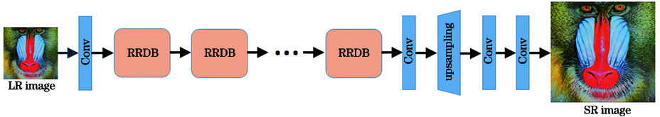
Fig. 1. Structure of the generator

Download full size

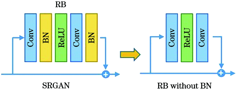
Fig. 2. Network structure after removing the BN layer

Download full size

Fig. 3. Structure of the RRDB

Download full size

Fig. 4. Structure of the discriminator

Download full size

Fig. 5. Schematic diagram of the training process. (a) Actual training curve; (b) ideal training curve^[16]

Download full size

Fig. 6. Training environment of the network

Download full size

Fig. 7. Interface of the MOI test system

Download full size

Fig. 8. PSNR of different algorithms in the Set5 test set

Download full size

Fig. 9. SSIM of different algorithms on the Set5 test set

Download full size

Fig. 10. PSNR of different algorithms on the Set14 test set

Download full size

Fig. 11. SSIM of different algorithms in the Set14 test set

Download full size

Fig. 12. Reconstruction effects of two algorithms. (a) Original image; (b) SRGAN algorithm; (c) our algorithm

Download full size

Fig. 13. Reconstruction results of 5 different algorithms. (a) Overall original image; (b) bicubic interpolation algorithm;(c) SRCNN algorithm; (d) VDSR algorithm; (e) SRResNet algorithm; (f) our algorithm; (g) partial original image

Download full size

Fig. 14. Railroad track image reconstructed by 5 different algorithms. (a) Overall original image; (b) bicubic interpolation algorithm; (c) SRCNN algorithm; (d) VDSR algorithm; (e) SRResNet algorithm; (f) our algorithm; (g) partial original image

Download full size

Evaluation standard	Score
No change in image quality	5
Slight change in image quality can be seen	4
Slightly hinder viewing	3
Hinder viewing	2
Seriously obstructing viewing	1

Table 1. Evaluation standard of the image quality

Relative measurement scale	Score
Quality is the worst in this picture group	1
Quality is below average in this picture group	2
Quality is on average in this picture group	3
Quality is above average in this picture group	4
Quality is the best in this picture group	5

Table 2. Scoring table for subjective evaluation of image quality

Algorithm	SRGAN^[13]	Ours	Difference
PSNR/dB	28.74	29.60	↑0.86
SSIM	0.8435	0.8558	↑0.0123

Table 3. Test results of different algorithms on the Set5 data set

Algorithm	SRGAN^[13]	Ours	Difference
PSNR/dB	25.75	26.44	↑0.69
SSIM	0.7370	0.7460	↑0.0090

Table 4. Test results of different algorithms on the Set14 data set

Algorithm	SRGAN^[13]	Ours	Difference
PSNR/dB	24.65	25.55	↑0.90
SSIM	0.6502	0.6549	↑0.0047

Table 5. Test results of different algorithms on the BSD100 data set

Data set	SRGAN(with BN)			Ours(with BN)			SRGAN(without BN)			Ours(without BN)
Data set	PSNR /dB	SSIM	Time /s	PSNR /dB	SSIM	Time /s	PSNR /dB	SSIM	Time /s	PSNR /dB	SSIM	Time /s
Set5	28.69	0.8415	0.21	29.02	0.8489	0.20	29.25	0.8483	0.20	29.60	0.8547	0.18
Set14	24.96	0.7187	0.43	26.10	0.7233	0.39	25.67	0.7203	0.42	26.41	0.7398	0.38
BSD100	24.01	0.6488	0.45	25.15	0.6511	0.43	25.10	0.6503	0.44	25.52	0.6548	0.41

Table 6. Influence of BN layer on algorithm performance

Dataset	Algorithm	Bicubic	SRCNN^[2]	VDSR^[5]	SRResNet^[13]	Ours
	PSNR /dB	28.43	30.14	31.35	31.92	29.60
Set5	SSIM	0.8211	0.8647	0.8838	0.8998	0.8558
	MOI	1.44	2.4	3.18	3.28	4.66
	PSNR /dB	25.99	27.18	28.01	28.39	26.44
Set14	SSIM	0.7486	0.7861	0.7674	0.8116	0.746
	MOI	1.42	2.43	3.18	3.59	4.38
	PSNR /dB	25.96	26.9	27.29	27.52	25.55
BSD100	SSIM	0.6675	0.7101	0.7251	0.7603	0.6549
	MOI	1.36	2.45	3.2	3.57	4.42

Table 7. Performance of different algorithms under three data sets

Download Citation

Set citation alerts for the article

Tools

Set citation alerts for the article

Save the article for my favorites

Paper Information