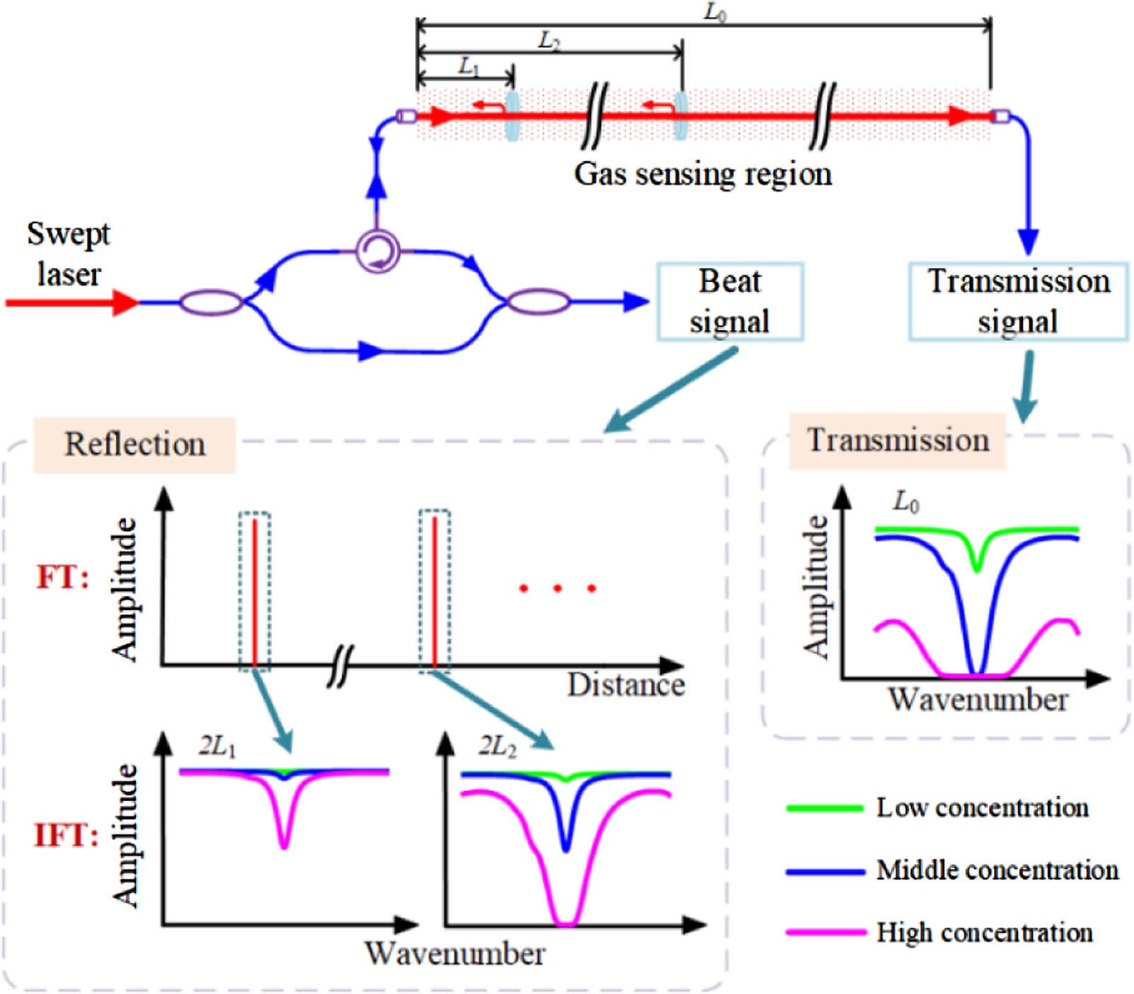
Fig. 1. Basic principle of OPMAS. The upper part is the basic configuration including an FMCW interferometer equipped with a gas cell having multiple internal reflections. The lower part is the procedure for the retrieval of spectral signals with different absorption pathlengths.

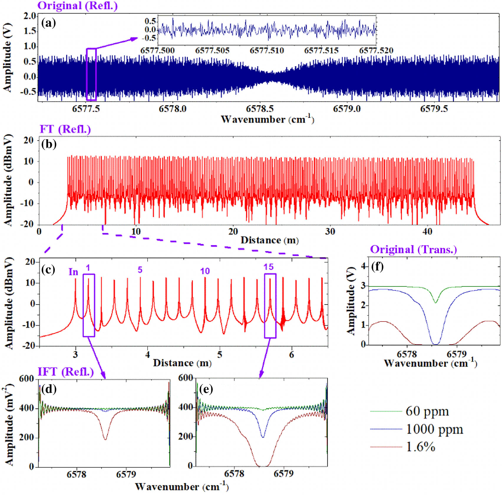
Fig. 2. Simulation of spectral signal retrievals with different OPLs using an MPC. (a) Original reflection-mode beat signals in spectral domain for 1000 ppm acetylene gas. The inset shows the local details of the beat signal. (b) DFT results in spatial domain containing 233 RPs. (c) Enlargement of the beginning part of (b). (d), (e) Retrieved spectral signals from two RPs (#1 and #15) for three different gas concentrations (60 ppm, 1000 ppm, and 1.6%). (f) Simulated spectral signals in the transmission mode.

Fig. 3. Experimental setup of the OPMAS. FRM, Faraday rotation mirror; PC, polarization controller; BPD, balanced photodetector; ATT, optical attenuator; DAQ, data acquisition.

Fig. 4. Experimental results of spectral signal retrieval at different reflection points in the MPC filled with 9250 ppm acetylene. (a) Acquired raw beat signals. (b) DFT of the signals shown in (a) with 50 results averaged. (c), (d) Enlargements of the beginning and end parts of (b). (e), (f) Spectral signals retrieved by IDFT from the RPs #1 and #13 shown in (c).

Fig. 5. Measured and simulated transmission spectra of acetylene at different concentrations with different absorption pathlengths. (a)–(d) For acetylene concentrations of 9.8%, 9250 ppm, 1120 ppm, and 95 ppm, with absorption pathlengths of 0.359 m, 0.359 m, 4.322 m, and 19.449 m, respectively.

Fig. 6. Measurement results of 9.3 ppm acetylene in the transmission mode. (a) Original transmission signal acquired in one period of the laser scan. (b) Measured transmission spectrum with 10 scans averaged and the corresponding HITRAN-simulated result.

Fig. 7. Plot of α(ν0) value versus gas concentration. Each error bar, magnified 10 times for clarity, shows the SD of five measurement results.

Table 1. Details of Experimental Data Used for Evaluating the Dynamic Range of Gas Sensing

Table 2. Comparison of Typical State-of-the-Art Laser Spectroscopic Gas Sensors