Experimental Study on Spatial Filtering Imaging Method of Diffraction Gratings

Xu Gao; Renjie Wang; Jinhuan Li; Yuting Wang; Jipeng Huang

doi:10.3788/AOS201838.0205001

Journals >Acta Optica Sinica >Volume 38 >Issue 2 >Page 0205001 > Article

Acta Optica Sinica
Vol. 38, Issue 2, 0205001 (2018)

Experimental Study on Spatial Filtering Imaging Method of Diffraction Gratings

Xu Gao^1、*, Renjie Wang², Jinhuan Li², Yuting Wang², and Jipeng Huang²

Author Affiliations

¹ School of Optoelectronic Engineering, Changchun University of Science and Technology, Changchun, Jilin 130022, China

² School of Physics, Northeast Normal University, Changchun, Jilin 130024, China

show less

DOI: 10.3788/AOS201838.0205001 Cite this Article Set citation alerts

Xu Gao, Renjie Wang, Jinhuan Li, Yuting Wang, Jipeng Huang. Experimental Study on Spatial Filtering Imaging Method of Diffraction Gratings[J]. Acta Optica Sinica, 2018, 38(2): 0205001 Copy Citation Text

show less

$Diffraction principle of photographic encoder grating signal. (a) Schematic of the head of an encoder; (b) propagation of light diffraction$

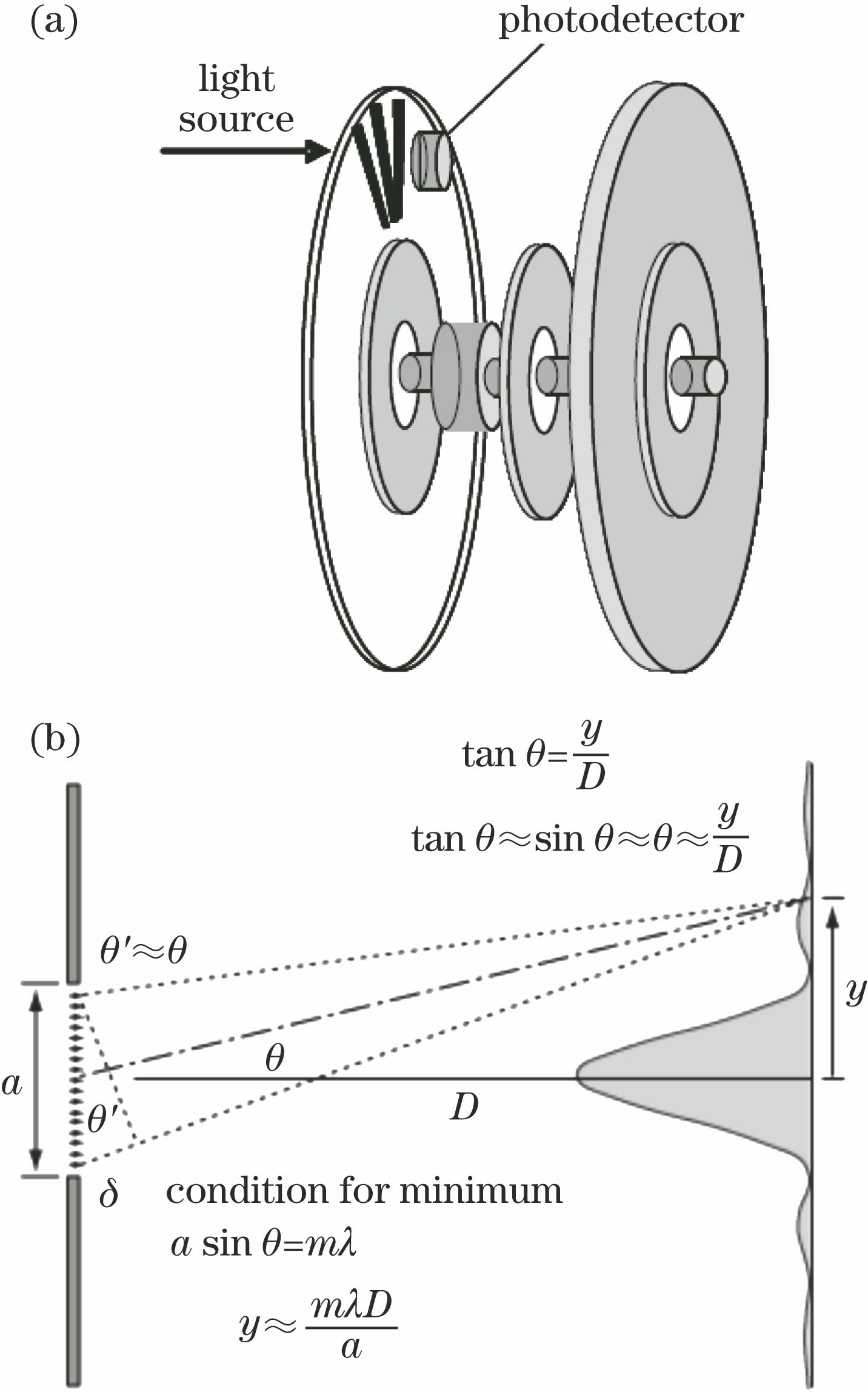
Fig. 1. Diffraction principle of photographic encoder grating signal. (a) Schematic of the head of an encoder; (b) propagation of light diffraction

Download full size

$Fraunhofer diffraction intensity distribution of rectangular grating$

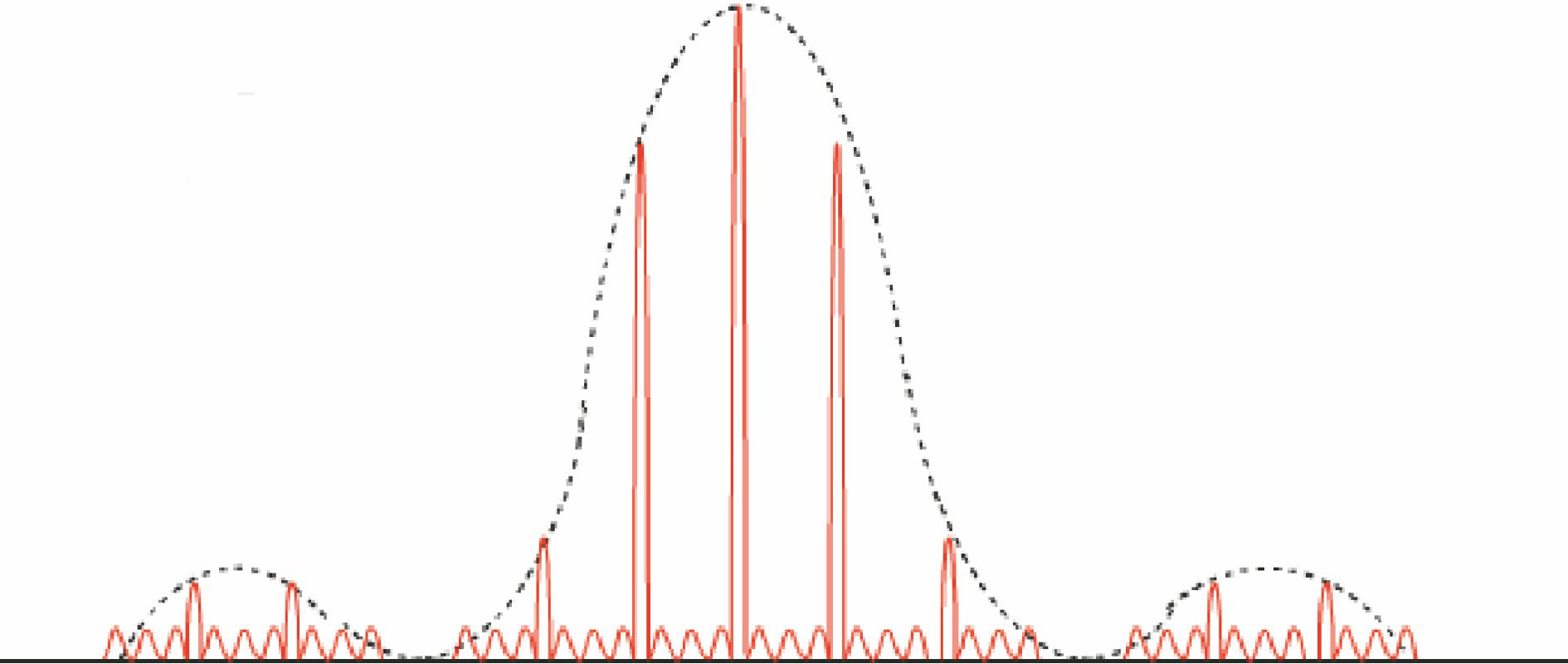
Fig. 2. Fraunhofer diffraction intensity distribution of rectangular grating

Download full size

Fig. 3. Optical design principle of sine holographic grating

Download full size

$Diffraction pattern of holographic grating and spatial frequency detection$

Fig. 4. Diffraction pattern of holographic grating and spatial frequency detection

Download full size

$Fraunhofer diffraction pattern of holographic grating$

Fig. 5. Fraunhofer diffraction pattern of holographic grating

Download full size

Fig. 6. Spatial filtering principle of grating

Download full size

$Fraunhofer diffraction pattern of filtered holographic gratings$

Fig. 7. Fraunhofer diffraction pattern of filtered holographic gratings

Download full size

Fig. 8. Optical system principle of grating test using parallel light

Download full size

Fig. 9. Optical system for testing grating using point light

Download full size

Fig. 10. Fringe images of multi-beam interferometry holographic grating with spatial frequency of 100 lp/mm before and after filtering imaging processing. (a) Before filtering; (b) after filtering

Download full size

Fig. 11. Transmittance functions of multi-beam interferometry holographic grating with spatial frequency of 100 lp/mm before and after filtering imaging processing. (a) Before filtering; (b) after filtering

Download full size

Fig. 12. Frequency spectra of multi-beam interferometry holographic grating with spatial frequency of 100 lp/mm before and after filtering imaging processing. (a) Before filtering; (b) after filtering

Download full size

$Diffraction light intensity distributions of multi-beam interferometry holographic grating with spatial frequency of 100 lp/mm before and after filtering imaging processing. (a) Before filtering; (b) after filtering$

Fig. 13. Diffraction light intensity distributions of multi-beam interferometry holographic grating with spatial frequency of 100 lp/mm before and after filtering imaging processing. (a) Before filtering; (b) after filtering

Download full size

Fig. 14. Frequency spectra of rectangular grating with spatial frequency of 100 lp/mm before and after filtering. (a) Before filtering; (b) after filtering

Download full size

$Diffraction light intensity distribution of rectangular grating with spatial frequency of 100 lp/mm$

Fig. 15. Diffraction light intensity distribution of rectangular grating with spatial frequency of 100 lp/mm

Download full size

$Diffraction light intensity distributions of rectangular grating with spatial frequency of 100 lp/mm after spatial filtering imaging processing. (a) Light intensity of -1 level and 0 level; (b) light intensity of 0 level and +1 level$

Fig. 16. Diffraction light intensity distributions of rectangular grating with spatial frequency of 100 lp/mm after spatial filtering imaging processing. (a) Light intensity of -1 level and 0 level; (b) light intensity of 0 level and +1 level

Download full size

Method	Advantage	Disadvantage
Fresnel double sided mirror and biprism	1) Fewer components;2) Symmetrical optical system and the optical path difference is almost zero;3) The range of the grating constant is wide	1) The light spot of interference area is small when using collimating lens;2) Two light beams are non-parallel without collimating lens
Lloyd mirror method	1) Fewer components and no secondary images;2) Simple operation and convenient adjustment	1) Relatively high requirements for the reflectivity of the reflector, collimation property of two light beams and the intensity ratio;2) Only suitable for the fabrication of gratings with larger constant and smaller spatial frequency;3) The interferential light beams are not strictly parallel
Michelson interferometry method	1) Larger size of the grating fabricated;2) Two-dimensional grating fabricated by one exposure	1) More transmissive components, so that the wave surface of the plane wave will be deformed and deviate from the plane wave;2) Only suitable for the fabrication of gratings with larger constant
Mach-Zehnder interferometry method	1) Symmetrical optical system and convenient to set up;2) The optical path difference of two light beams is small and the interference effect is good;3) The adjustment is convenient and the spatial frequency of gratings can be changed with the adjustment of one beam splitter angle	1) More optical components and the fringe is uneven and the symmetry property is decreased;2) The angle between the reflected light and the transmissive light is small and the grating constant is not accurate;3) The angle of two light beams is restricted by the area of beam splitter and this method is not suitable for the fabrication of gratings with small constant

Table 1. Advantages and disadvantages of sine grating fabrication method

$\begin{matrix} {f_{0}}_{} \end{matrix}$ /(lp·mm^-1)	50	100	120	150
$\begin{matrix} {d_{0}}_{} \end{matrix}$ /cm	0.791	1.582	1.898	2.373

Table 2. Relationship between d0 and f0

f″₀ /(lp·mm^-1)	50	100	120	150
p /cm	1.265	2.531	3.037	3.797

Table 3. Relationship between f″0 and p

f″ $\begin{matrix} {_{0}}_{} \end{matrix}$ /(lp·mm^-1)	50	100	120	150
p /cm	2.530	5.065	6.075	7.600
f″ $\begin{matrix} {_{1}}_{} \end{matrix}$ /(lp·mm^-1)	100	200	240	300

Table 4. Relationship among f″0, f″1, and p

$\begin{matrix} y_{100}^{\pm 1} \end{matrix}$	$\begin{matrix} y_{100}^{\pm 2} \end{matrix}$	p₁₀₀	$\begin{matrix} {\bar{p}}_{100} \end{matrix}$
100	5.3850	0.0539
110	5.6617	0.0515
120	6.3600	0.0530
130	6.8419	0.0526
140	7.3262	0.0523
150	7.3800	0.0492	0.0527
160	8.2240	0.0514
170	8.8315	0.0520
180	9.6426	0.0536
190	9.8705	0.0520
200	11.6800	0.0584

Table 5. Light intensity ratio of ±2 level to ±1 level of grating with spatial frequency of 100 lp/mm

Spatial frequency /(lp·mm^-1)	50	100	120	150
Light intensity ratio /%	8.59	5.27	3.50	2.48

Table 6. Light intensity ratio of ±2 level to ±1 level of each grating

Xu Gao, Renjie Wang, Jinhuan Li, Yuting Wang, Jipeng Huang. Experimental Study on Spatial Filtering Imaging Method of Diffraction Gratings[J]. Acta Optica Sinica, 2018, 38(2): 0205001

Download Citation

Set citation alerts for the article

Tools

Set citation alerts for the article

Save the article for my favorites

Paper Information