
Mingrui YANG, Qizheng SUN, Chixu LUO, Donghao HE, Xiaojing LIU, Tengfei ZHANG. Development and verification of a neutronics-thermal hydraulics coupling code with unstructured meshes neutron transport model[J]. NUCLEAR TECHNIQUES, 2023, 46(3): 030601
- NUCLEAR TECHNIQUES
- Vol. 46, Issue 3, 030601 (2023)
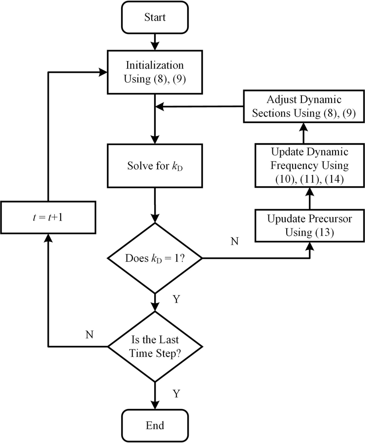
Fig. 1. Flowchart of the transient calculations with SCM in MORPHY

Fig. 2. Channel equivalent diagram
Fig. 3. The coupling method in MORPHY (a) OSSI method, (b) FPI method
Fig. 4. Layout of the TWIGL benchmark problem
Fig. 5. Results of the TWIGL A1 (a), A2 (b) problem
Fig. 6. Layout of the Dodds problem (a) Material layout, (b) Radial mesh generation
Fig. 7. Dodds benchmark problem relative power vs. time
Fig. 8. Layout of the NEACRP benchmark problem
Fig. 9. NEACRP benchmark problem relative power vs. time (a) NEACRP A1, (b) NEACRP A2, (c) NEACRP B1, (d) NEACRP B2
Fig. 10. NEACRP benchmark power distribution at peak power
| ||||||||||||||||||||||||||||||||||||||||||||
Table 1. Comparison of core relative powers for the TWIGL A1 problem
| ||||||||||||||||||||||||||||||||||||||||||||
Table 2. Comparison of core relative powers for the TWIGL A2 problem
| |||||||||||||||||||||||||||||||||||||||||||||||||||||||||||||||||||||||
Table 3. Comparison of steady-state results for NEACRP problems
|
Table 4. Peak power at different time-step sizes for OSSI method
|
Table 5. Peak power of different thermal-hydraulic time-step sizes using FPI method in case A1
| ||||||||||||||||||||||||||||||||||||||||||||||||||||||
Table 6. Comparison of MORPHY A1 and A2 results with PARCS

Set citation alerts for the article
Please enter your email address
© Copyright 2018-2021 | Chinese Laser Press. All Rights Reserved 沪ICP备15018463号-20