
Xin Wang, Yuan Sun, Liang Liu, "Realizing fast temperature measurement and simulating Maxwell’s demon with nearly nondestructive detection in cold atoms," Photonics Res. 10, 1947 (2022)
- Photonics Research
- Vol. 10, Issue 8, 1947 (2022)
Abstract
1. INTRODUCTION
Temperature is an essential topic in laser cooling of atoms [1,2], ions [3,4], molecules [5–7], solids [8–11], and cavity optomechanical systems [12–14]. The rapid development of quantum technologies with cold atom ensembles, including quantum precision measurement [15–17], quantum sensing [18], quantum simulation [19–21], and quantum information [22,23], raises emerging requirements for fast temperature measurement with minimal disturbance and an effective method of sorting out relatively colder atoms. However, the routine technique of time-of-flight (TOF) [24–27] is a destructive detection method that usually costs about a few tens to hundreds of milliseconds. Nondestructive thermometry has been developed for typical cold atom systems of optical molasses [28,29], optical dipole traps [30], and Bose–Einstein condensates (BECs) [31], and yet these methods still need significantly more than 1 ms data acquisition time in practice.
On the other hand, the idea of filtering colder atoms has profound connections with the concept of Maxwell’s demon, which is an imagined creature with the ability of identifying particles with smaller velocities and subsequently separating them from the hotter ones [32]. Experiments with Maxwell’s demon-type behavior have already been proposed and demonstrated in various systems [33–41]. For cold atoms, 1D quasi-single-velocity cooling [42] and one-way potential barriers for the optical dipole trap [43] have been realized. Nevertheless, generic Maxwell’s demon-type operation of identifying atoms with smaller velocity values remains elusive in cold atom systems. Meanwhile, lower temperature often implies longer coherence time and better precision, especially in cold atom clock [44] and ultracold atom interferometry [45]; therefore, sorting out the relatively colder portion of a cold atom ensemble is not only theoretically interesting but also practically helpful.
In this paper, we first demonstrate deterministic measurement of temperature within less than 1 ms detection time and effective filtering of colder atoms with temperature less than 1 μK starting from an ensemble with about 20 μK. The essential procedure consists of a well calibrated labeling operation of atoms and nearly nondestructive detection with continuous optical pulses, relying on the polarization control of the atoms’ internal states and a cycling transition. Our method is compatible with various types of cold atom platforms, and here we choose isotropic laser cooling (ILC) [46–49] due to its advantage of generating cold atoms with nearly perfect isotropic thermal properties in all three dimensions. It is attainable to acquire information of temperature within 1 ms because the absorption change of probe laser is obviously distinguishable in theory even for cold atoms with very low temperature, when the signal-to-noise ratio is adequate. Then we move on to discuss sorting out the colder portion of labeled atoms, which amounts to mapping velocity distribution into spatial distribution over a few tens of milliseconds. Finally, we show that, by tuning the labeling process, whether the atom passing by the region of labeling lasers gets transferred to state will become dependent on its velocity. This almost reproduces the original thought experiment of a Maxwell’s demon labeling the atoms according to their velocities, where the label is now instantiated in terms of the atomic internal states.
Sign up for Photonics Research TOC. Get the latest issue of Photonics Research delivered right to you!Sign up now
2. METHODS
The basic experimental setup is depicted in Fig. 1(a). The labeling lasers consist of the polarizing laser, which drives the population among
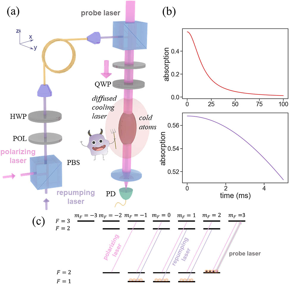
Figure 1.(a) Schematic of the experiment. The cold atom ensemble is prepared by a uniformly diffused cooling laser. A polarizing beam splitter (PBS), polarizers (POL), and a half-wave plate (HWP) are employed to combine the polarizing laser and the repumping laser for the labeling process. A quarter-wave plate turns the labeling lasers and the probe laser into circular polarization. The probe laser propagates and eventually arrives at a photodetector (PD). The labeling lasers and probe laser are concentric and aligned along the direction of gravity. No bias magnetic field is required. (b) Theory curve of the absorption signal for cold atoms of 20 μK as the 2D temperature. (c) Relevant energy levels of
The density profile of labeled atoms will vary over time due to the diffusion related with their kinematic motions, and such a change can be revealed in the absorption signal of the probe laser in the form of bucket detection. The velocity distribution of these laser cooled atoms has been already identified as the Maxwell–Boltzmann distribution in previous experimental investigations [28,50], which corroborated the general theory of laser cooling [51]. Moreover, it is known that the cold atom density is reasonably uniform in the central region of ILC [52,53]. With these information as
The details of derivation will be discussed later in Section 3.A. Here,
A sample theory curve of Eq. (1) is shown in Fig. 1(b). We observe that the derivative is changing rapidly during the beginning few milliseconds, and this feature makes it possible to measure temperature on a time scale less than 1 ms. Namely, even for a small time duration, the bucket detection of the probe laser can effectively deduce the temperature, according to the density change due to the thermal motion of cold atoms.
ILC is usually realized in the form of generating cold atoms by diffuse reflection light [49,54–56]. Its operation requires neither the careful alignment of cooling lasers or the presence of magnetic gradient field, and it is known for the characteristics of compactness and robustness. The implementation of ILC usually relies on an all-optical structure with the surface of vacuum chamber coated with diffuse reflective material.
For our ILC process, the cooling lasers consist of the main cooling laser and the secondary repumping laser. The main cooling laser is typically red detuned by 20–25 MHz to the transition of
In order to realize the nearly nondestructive detection, it requires a proper time sequence of experiment. The sample time sequences of the fast temperature measurement and simulating Maxwell’s demon experiments are demonstrated in Figs. 2 and 3, respectively. In particular, immediately after the cooling lasers are turned off, a pumping laser will optically pump all the cold atoms to the
![]()
Figure 2.Sample time sequence for our experiment of fast temperature measurement with nearly nondestructive detection. The pumping laser is resonant with the transition of
![]()
Figure 3.Sample time sequence for our experiment of simulating Maxwell’s demon in terms of velocity-dependent labeling. A mechanical shutter is employed to ensure the labeling lasers are stopped completely, such that we intentionally keep a waiting period up to several milliseconds at the end of cooling stage for it to stabilize, which is not necessary in theory. We omit this extra gap time in this graph.
3. THEORY
A. Relation between the Time-Dependent Absorption Signal and Temperature
Here we discuss the detailed derivation of how to deduce the temperature of labeled cold atoms from the absorption signal of the probe laser in the form of bucket detection. In particular, the issue of finite labeling area determined by the labeling lasers will be specifically addressed.
First, we review the idealized case that the labeled atoms take the form of a thin line with zero width along the
If we define an artificial proportionality constant
Inevitably, the thin line description is oversimplified for the actual situation encountered in experimentation, especially during the beginning phase of a few milliseconds immediately after the labeling process. In order to take the finite labeling area into consideration, we assume a uniform physical density of the cold atoms near the central region, which is a reasonable thing to expect for ILC [46–49,52,53]. Then the absorption of the probe laser includes the contributions of cold atoms traveling from all possible originates within the effective labeling area. According to this viewpoint, the transmission can be calculated as
The above expression leaves us to evaluate an integral in the form of
As in Eq. (1), we adopt the two parameters
Since Eq. (7) describes the transmitted light, and therefore in the polar coordinate system, the absorption of light is proportional to
When Eq. (1) is employed in the fitting process to extract the value of temperature, typically it will only need two free parameters: constant and
In Fig. 4, we show a few typical theory curves with emphasis put on the first few milliseconds immediately after the labeling process. From the behavior of curves associated with different temperature values, we observe that
![]()
Figure 4.Theory curves according to Eq. (
B. Filtering Out the Colder Part of Labeled Atoms
Once the labeling procedure is accomplished, the labeled atoms staying within the region defined by the probe laser become colder and colder as time elapses since the hotter atoms gradually leave the region. Such a process effectively behaves like filtering out the colder atoms.
Here we discuss the details about how to quantitatively describe such a process. As in the previous analysis, the derivations will be put under the 2D framework in the
With these preparations, we can express
In order to comply with the typical situation with circular symmetry, we can reformulate Eq. (11) into a format with specific individual integral limits in the polar coordinates. And, eventually, with the interpretations that
Although Eq. (13) cannot be further reduced to an analytical form, it can be evaluated by numerical integration methods, as we will show later in Section 4.
C. Velocity-Dependent Labeling Process
Here we discuss a few more theoretical details about simulating the Maxwell’s demon thought experiment with the velocity-dependent labeling process.
The essence is to investigate the relation between averaged number of scattering events in the optical pumping process toward the destination state of
Initially, the atomic population is evenly distributed among the three states:
Therefore, in such a simplified picture, on average it takes one scattering event of the repumping laser and one scattering event of the polarizing laser to reach the destination of
On the other hand, a more rigorous approach needs to include the details of spontaneous emissions and the nuances of different Zeeman sub-states. The Monte Carlo wave function (MCWF) method serves well for this purpose, and we briefly discuss the basic formalism here. We begin with the equations of motion for the atomic wave functions without decay. According to the linkage structure of the atomic transitions that we have chosen, under the rotating wave approximation, the time evolution of the wave function can be expressed in terms of ordinary differential equations. For the wave function, we use the notation of
Rabi Frequencies for the Transitions Associated with the Repumping Laser in the Labeling Interaction Process
| Ωj | |||
|---|---|---|---|
| 1 | |||
| 2 | |||
| 3 |
The Rabi frequency
Rabi Frequencies for the Transitions Associated with the Polarizing Laser in the Labeling Interaction Process
| Ωj | |||
|---|---|---|---|
| 4 | |||
| 5 | |||
| 6 | |||
| 7 | |||
| 8 |
The Rabi frequency
Then, the ordinary equation system can be expressed in terms of
Next, the spontaneous emission can be treated as quantum jumps with the help of the pseudorandom number generators, according to the framework of MCWF method. The destination of spontaneous emission can be set as the randomized linear superposition of physically allowed states in the ground level, in order to better emulate the optical pumping effects. After running many such MCWF trajectories, the averaged numerical result will become a reasonable explanation of the velocity-dependent labeling process.
4. RESULTS AND DISCUSSION
A typical experimental result is shown in Fig. 5, where the absorption signal is collected from a single continuous pulse of probe laser and the data point is recorded every 5 μs. Here, the radius of labeled area
![]()
Figure 5.Obtain temperature from a single trace of experimental data, costing less than 1 ms. The inset shows the details of the first 200 μs. This probe laser pulse starts at 3.3 ms after the labeling process, mostly because of waiting for the mechanical shutter of labeling lasers to fully close. The method of trust region reflective is employed for the fitting.
In order to verify our description of the dynamics, especially on a relatively large time scale, we further carry out the experiment with two short probe pulses separated by tens of milliseconds. In fact, such a dual-pulse measurement is made possible by the nearly nondestructive detection, as the first probe pulse does not disturb the labeled cold atoms or cause excessive heating. In Fig. 6, we demonstrate a representative result, together with a fitting to the overall data according to Eq. (1). We observe that the global fitting curve agrees well with the experimental data locally for both pulses, which supports the accuracy of temperature measurement with less than 1 ms data taken very soon after the labeling operation. We repeat this type of dual-pulse experiment multiple times with different initial temperatures ranging from 10 μK to 30 μK, and similar to the situation of Fig. 6, the outcomes are consistent with our anticipations.
![]()
Figure 6.Result of dual-pulse experiment, obtained from a single experimental trial. The inset shows the detailed data of the two pulses, respectively. Here the radius of labeled area
Moreover, we can vary the delay times in the dual-pulse experiment. In Fig. 6, we have intentionally presented the experimental result with a relatively long delay time in order to show the effects of velocity filtering. On the other hand, we can certainly choose a shorter delay time, as shown in Fig. 7. Again, we observe that the global fitting curve agrees well with the experimental data.
![]()
Figure 7.Result of dual-pulse experiment with a relatively short time delay between the two probe pulses.
In the derivation of Eq. (1), the kinematic motions of labeled cold atoms along the
On the other hand, the result of Fig. 6 can be interpreted from an alternative viewpoint that the hotter atoms quickly leave the region defined by the probe laser while the cooler atoms tend to stay longer. Therefore, the dual-pulse experiment can behave as an effective method to filter out the colder part of the labeled atoms, where the nondestructive detection serves an indicator of the filtering process. As time elapses, the velocities of leftover labeled atoms gradually deviate from the Maxwell–Boltzmann distribution while the idea of thermal equilibrium apparently does not apply; therefore, the concept of temperature requires careful clarifications. Here we calculate the temperature as the averaged kinematic energies of the
![]()
Figure 8.Theory curve that describes the filtering of colder atoms in terms of 2D temperature, with
Our implementation of filtering has been limited to the 2D setting. If a fully 3D result is wanted, then extra operations need be applied to the dynamics of
Next, we turn our attention back to the labeling process. Previously, its role was limited to quickly optically pumping the cold atoms within a prescribed region to the specific target state
![]()
Figure 9.(a) Cartoon of atoms traveling through the region of labeling lasers, which leads to velocity-dependent labeling. (b) Relation between
We estimate the velocity dependence of such labeling processes in a simplified way. On average, it takes one scattering event of the repumping laser and one scattering event of the polarizing laser to reach
We proceed with measurements according to the above discussions, with a larger cooling laser power such that the atoms begin with 2D temperature much higher than that of Fig. 5. In particular, we set the labeling interaction time as
ILC leads to relatively dilute cold atom gases; therefore, we have carefully suppressed the intensity and frequency noises of probe laser in order to obtain a good signal-to-noise ratio, which is vital in the temperature measurement process as can be seen in discussions of Section 3. While we have demonstrated so far that our experiments behave for such a dilute gas OD on the order of 1 or even less, we have also set up experimental tests to verify that it works well for cold atom ensembles with much higher density, and in particular with respect to a high density cold atom ensemble prepared via 3D magneto-optical trap (MOT). The preliminary testing results suggest that we have obtained essentially the same kind of behavior in the outcome. In particular, a cold atom ensemble with higher OD reduces the requirements on the probe laser.
In fact, since the velocity of cold atoms almost stays unchanged during the process, the analysis of entropy can be established by paying attention only to the internal degrees of freedom. In such a simplified picture, we assume that here exist two different states of
5. CONCLUSION
In summary, we propose and demonstrate sub-millisecond temperature measurement of labeled cold atoms by a single continuous probe pulse in the form of nearly nondestructive detection. We further utilize this method to show that it is possible to filter out the sub-μK part from labeled atoms of tens of μK in a straightforward way, evaluated in the
Acknowledgment
Acknowledgment. The authors gratefully acknowledge support from the National Natural Science Foundation of China, the National Key R&D Program of China, and the Chinese Academy of Sciences, the China Manned Space Engineering Office. The authors also thank Ning Chen, Yanling Meng, Peng Xu, and Xiaodong He for helpful discussions.
References
[1] W. D. Phillips, H. Metcalf. Laser deceleration of an atomic beam. Phys. Rev. Lett., 48, 596-599(1982).
[2] S. Chu, L. Hollberg, J. E. Bjorkholm, A. Cable, A. Ashkin. Three-dimensional viscous confinement and cooling of atoms by resonance radiation pressure. Phys. Rev. Lett., 55, 48-51(1985).
[3] F. Diedrich, J. C. Bergquist, W. M. Itano, D. J. Wineland. Laser cooling to the zero-point energy of motion. Phys. Rev. Lett., 62, 403-406(1989).
[4] J. I. Cirac, P. Zoller. Quantum computations with cold trapped ions. Phys. Rev. Lett., 74, 4091-4094(1995).
[5] I. Kozyryev, L. Baum, K. Matsuda, B. L. Augenbraun, L. Anderegg, A. P. Sedlack, J. M. Doyle. Sisyphus laser cooling of a polyatomic molecule. Phys. Rev. Lett., 118, 173201(2017).
[6] J. Lim, J. R. Almond, M. A. Trigatzis, J. A. Devlin, N. J. Fitch, B. E. Sauer, M. R. Tarbutt, E. A. Hinds. Laser cooled YbF molecules for measuring the electron’s electric dipole moment. Phys. Rev. Lett., 120, 123201(2018).
[7] L. Baum, N. B. Vilas, C. Hallas, B. L. Augenbraun, S. Raval, D. Mitra, J. M. Doyle. 1D magneto-optical trap of polyatomic molecules. Phys. Rev. Lett., 124, 133201(2020).
[8] R. I. Epstein, M. I. Buchwald, B. C. Edwards, T. R. Gosnell, C. E. Mungan. Observation of laser-induced fluorescent cooling of a solid. Nature, 377, 500-503(1995).
[9] S. D. Melgaard, D. V. Seletskiy, A. D. Lieto, M. Tonelli, M. Sheik-Bahae. Optical refrigeration to 119 K, below National Institute of Standards and Technology cryogenic temperature. Opt. Lett., 38, 1588-1590(2013).
[10] P. B. Roder, B. E. Smith, X. Zhou, M. J. Crane, P. J. Pauzauskie. Laser refrigeration of hydrothermal nanocrystals in physiological media. Proc. Natl. Acad. Sci. USA, 112, 15024-15029(2015).
[11] A. T. M. A. Rahman, P. F. Barker. Laser refrigeration, alignment and rotation of levitated Yb3+:YLF nanocrystals. Nat. Photonics, 11, 634-638(2017).
[12] Q. Lin, J. Rosenberg, X. Jiang, K. J. Vahala, O. Painter. Mechanical oscillation and cooling actuated by the optical gradient force. Phys. Rev. Lett., 103, 103601(2009).
[13] G. S. Wiederhecker, L. Chen, A. Gondarenko, M. Lipson. Controlling photonic structures using optical forces. Nature, 462, 633-636(2009).
[14] M. Aspelmeyer, T. J. Kippenberg, F. Marquardt. Cavity optomechanics. Rev. Mod. Phys., 86, 1391-1452(2014).
[15] A. Derevianko, H. Katori. Colloquium: physics of optical lattice clocks. Rev. Mod. Phys., 83, 331-347(2011).
[16] W. Ren, T. Li, Q. Qu, B. Wang, L. Li, D. Lü, W. Chen, L. Liu. Development of a space cold atom clock. Natl. Sci. Rev., 7, 1828-1836(2020).
[17] B. Chen, J. Long, H. Xie, C. Li, L. Chen, B. Jiang, S. Chen. Portable atomic gravimeter operating in noisy urban environments. Chin. Opt. Lett., 18, 090201(2020).
[18] C. L. Degen, F. Reinhard, P. Cappellaro. Quantum sensing. Rev. Mod. Phys., 89, 035002(2017).
[19] J. Dalibard, F. Gerbier, G. Juzeliūnas, P. Öhberg. Colloquium: artificial gauge potentials for neutral atoms. Rev. Mod. Phys., 83, 1523-1543(2011).
[20] R. A. Hart, P. M. Duarte, T.-L. Yang, X. Liu, T. Paiva, E. Khatami, R. T. Scalettar, N. Trivedi, D. A. Huse, R. G. Hulet. Observation of antiferromagnetic correlations in the Hubbard model with ultracold atoms. Nature, 519, 211-214(2015).
[21] H. Bernien, S. Schwartz, A. Keesling, H. Levine, A. Omran, H. Pichler, S. Choi, A. S. Zibrov, M. Endres, M. Greiner, V. Vuletić, M. D. Lukin. Probing many-body dynamics on a 51-atom quantum simulator. Nature, 551, 579-584(2017).
[22] K. Hammerer, A. S. Sørensen, E. S. Polzik. Quantum interface between light and atomic ensembles. Rev. Mod. Phys., 82, 1041-1093(2010).
[23] M. Saffman, T. G. Walker, K. Mølmer. Quantum information with Rydberg atoms. Rev. Mod. Phys., 82, 2313-2363(2010).
[24] D. S. Weiss, E. Riis, Y. Shevy, P. J. Ungar, S. Chu. Optical molasses and multilevel atoms: experiment. J. Opt. Soc. Am. B, 6, 2072-2083(1989).
[25] R. Gati, B. Hemmerling, J. Fölling, M. Albiez, M. K. Oberthaler. Noise thermometry with two weakly coupled Bose-Einstein condensates. Phys. Rev. Lett., 96, 130404(2006).
[26] F. M. Spiegelhalder, A. Trenkwalder, D. Naik, G. Hendl, F. Schreck, R. Grimm. Collisional stability of 40 K immersed in a strongly interacting Fermi gas of 6Li. Phys. Rev. Lett., 103, 223203(2009).
[27] H. Cheng, S. Deng, Z. Zhang, J. Xiang, J. Ji, W. Ren, T. Li, Q. Qu, L. Liu, D. Lü. Uncertainty evaluation of the second-order Zeeman shift of a transportable 87Rb atomic fountain clock. Chin. Opt. Lett., 19, 120201(2021).
[28] X. Wang, Y. Sun, H.-D. Cheng, J.-Y. Wan, Y.-L. Meng, L. Xiao, L. Liu. Nearly nondestructive thermometry of labeled cold atoms and application to isotropic laser cooling. Phys. Rev. Appl., 14, 024030(2020).
[29] X. Wang, Y. Sun, L. Liu. Characterization of isotropic laser cooling for application in quantum sensing. Opt. Express, 29, 43435-43444(2021).
[30] P. G. Petrov, D. Oblak, C. L. G. Alzar, N. Kjærgaard, E. S. Polzik. Nondestructive interferometric characterization of an optical dipole trap. Phys. Rev. A, 75, 033803(2007).
[31] M. Mehboudi, A. Lampo, C. Charalambous, L. A. Correa, M. A. García-March, M. Lewenstein. Using polarons for sub-nK quantum nondemolition thermometry in a Bose-Einstein condensate. Phys. Rev. Lett., 122, 030403(2019).
[32] J. C. Maxwell. Theory of Heat(1871).
[33] V. Serreli, C.-F. Lee, E. R. Kay, D. A. Leigh. A molecular information ratchet. Nature, 445, 523-527(2007).
[34] S. Toyabe, T. Sagawa, M. Ueda, E. Muneyuki, M. Sano. Experimental demonstration of information-to-energy conversion and validation of the generalized Jarzynski equality. Nat. Phys., 6, 988-992(2010).
[35] J. V. Koski, V. F. Maisi, T. Sagawa, J. P. Pekola. Experimental observation of the role of mutual information in the nonequilibrium dynamics of a Maxwell demon. Phys. Rev. Lett., 113, 030601(2014).
[36] J. V. Koski, V. F. Maisi, J. P. Pekola, D. V. Averin. Experimental realization of a Szilard engine with a single electron. Proc. Natl. Acad. Sci. USA, 111, 13786-13789(2014).
[37] J. V. Koski, A. Kutvonen, I. M. Khaymovich, T. Ala-Nissila, J. P. Pekola. On-chip Maxwell’s demon as an information-powered refrigerator. Phys. Rev. Lett., 115, 260602(2015).
[38] M. D. Vidrighin, O. Dahlsten, M. Barbieri, M. S. Kim, V. Vedral, I. A. Walmsley. Photonic Maxwell’s demon. Phys. Rev. Lett., 116, 050401(2016).
[39] P. A. Camati, J. P. S. Peterson, T. B. Batalhão, K. Micadei, A. M. Souza, R. S. Sarthour, I. S. Oliveira, R. M. Serra. Experimental rectification of entropy production by Maxwell’s demon in a quantum system. Phys. Rev. Lett., 117, 240502(2016).
[40] N. Cottet, S. Jezouin, L. Bretheau, P. Campagne-Ibarcq, Q. Ficheux, J. Anders, A. Auffèves, R. Azouit, P. Rouchon, B. Huard. Observing a quantum Maxwell demon at work. Proc. Natl. Acad. Sci. USA, 114, 7561-7564(2017).
[41] R. Sánchez, J. Splettstoesser, R. S. Whitney. Nonequilibrium system as a demon. Phys. Rev. Lett., 123, 216801(2019).
[42] T. Binnewies, U. Sterr, J. Helmcke, F. Riehle. Cooling by Maxwell’s demon: preparation of single-velocity atoms for matter-wave interferometry. Phys. Rev. A, 62, 011601(2000).
[43] J. J. Thorn, E. A. Schoene, T. Li, D. A. Steck. Dynamics of cold atoms crossing a one-way barrier. Phys. Rev. A, 79, 063402(2009).
[44] L. Liu, D.-S. Lü, W.-B. Chen, T. Li, Q.-Z. Qu, B. Wang, L. Li, W. Ren, Z.-R. Dong, J.-B. Zhao, W.-B. Xia, X. Zhao, J. W. Ji, M.-F. Ye, Y.-G. Sun, Y.-Y. Yao, D. Song, Z.-G. Liang, S.-J. Hu, D.-H. Yu, X. Hou, W. Shi, H.-G. Zang, J.-F. Xiang, X.-K. Peng, Y.-Z. Wang. In-orbit operation of an atomic clock based on laser-cooled 87Rb atoms. Nat. Commun., 9, 2760(2018).
[45] G. M. Tino, A. Bassi, G. Bianco, K. Bongs, P. Bouyer, L. Cacciapuoti, S. Capozziello, X. Chen, M. L. Chiofalo, A. Derevianko, W. Ertmer, N. Gaaloul, P. Gill, P. W. Graham, J. M. Hogan, L. Iess, M. A. Kasevich, H. Katori, C. Klempt, X. Lu, L.-S. Ma, H. Müller, N. R. Newbury, C. W. Oates, A. Peters, N. Poli, E. M. Rasel, G. Rosi, A. Roura, C. Salomon, S. Schiller, W. Schleich, D. Schlippert, F. Schreck, C. Schubert, F. Sorrentino, U. Sterr, J. W. Thomsen, G. Vallone, F. Vetrano, P. Villoresi, W. von Klitzing, D. Wilkowski, P. Wolf, J. Ye, N. Yu, M. Zhan. SAGE: a proposal for a space atomic gravity explorer. Eur. Phys. J. D, 73, 228(2019).
[46] Y. Z. Wang. Atomic beam slowing by diffusive light in an integrating sphere(1979).
[47] W. Ketterle, A. Martin, M. A. Joffe, D. E. Pritchard. Slowing and cooling atoms in isotropic laser light. Phys. Rev. Lett., 69, 2483-2486(1992).
[48] H. Batelaan, S. Padua, D. H. Yang, C. Xie, R. Gupta, H. Metcalf. Slowing of 87Rb atoms with isotropic light. Phys. Rev. A, 49, 2780-2784(1994).
[49] M. Langlois, L. De Sarlo, D. Holleville, N. Dimarcq, J.-F. Schaff, S. Bernon. Compact cold-atom clock for onboard timebase: tests in reduced gravity. Phys. Rev. Appl., 10, 064007(2018).
[50] E. Guillot, P.-E. Pottie, N. Dimarcq. Three-dimensional cooling of cesium atoms in a reflecting copper cylinder. Opt. Lett., 26, 1639-1641(2001).
[51] H. J. Metcalf, P. van der Straten. Laser Cooling and Trapping(1999).
[52] X.-C. Wang, H.-D. Cheng, L. Xiao, B.-C. Zheng, Y.-L. Meng, L. Liu, Y.-Z. Wang. Measurement of spatial distribution of cold atoms in an integrating sphere. Chin. Phys. Lett., 29, 023701(2012).
[53] S. Trémine, E. de Clercq, P. Verkerk. Isotropic light versus six-beam molasses for Doppler cooling of atoms from background vapor: theoretical comparison. Phys. Rev. A, 96, 023411(2017).
[54] F.-X. Esnault, D. Holleville, N. Rossetto, S. Guerandel, N. Dimarcq. High-stability compact atomic clock based on isotropic laser cooling. Phys. Rev. A, 82, 033436(2010).
[55] P. Liu, Y. Meng, J. Wan, X. Wang, Y. Wang, L. Xiao, H. Cheng, L. Liu. Scheme for a compact cold-atom clock based on diffuse laser cooling in a cylindrical cavity. Phys. Rev. A, 92, 062101(2015).
[56] Y. Wang, Y. Meng, J. Wan, M. Yu, X. Wang, L. Xiao, H. Cheng, L. Liu. Optical-plus-microwave pumping in a magnetically insensitive state of cold atoms. Phys. Rev. A, 97, 023421(2018).
[57] W. D. Phillips. Nobel lecture: laser cooling and trapping of neutral atoms. Rev. Mod. Phys., 70, 721-741(1998).
[58] H. Metcalf. Entropy exchange in laser cooling. Phys. Rev. A, 77, 061401(2008).


Set citation alerts for the article
Please enter your email address

© Copyright 2018-2021 | Chinese Laser Press. All Rights Reserved 沪ICP备15018463号-20