• Opto-Electronic Engineering
  • Vol. 51, Issue 1, 230290-1 (2024)
Wenxue Zhang1、2、3、4, Yihan Luo1、2、3、4、*, Yaqing Liu1、2、3, Shiye Xia1、2、3, and Kaiyuan Zhao1、2、3、4
Author Affiliations
  • 1National Key Laboratory of Optical Field Manipulation Science and Technology, Chinese Academy of Sciences, Chengdu, Sichuan 610209, China
  • 2Key Laboratory of Beam Control, Chinese Academy of Sciences, Chengdu, Sichuan 610209, China
  • 3Institute of Optics and Electronics, Chinese Academy of Sciences, Chengdu, Sichuan 610209, China
  • 4University of Chinese Academy of Sciences, Beijing 100049, China
  • show less
    DOI: 10.12086/oee.2024.230290 Cite this Article
    Wenxue Zhang, Yihan Luo, Yaqing Liu, Shiye Xia, Kaiyuan Zhao. Image super-resolution reconstruction based on active displacement imaging[J]. Opto-Electronic Engineering, 2024, 51(1): 230290-1 Copy Citation Text show less
    The image degradation process
    Fig. 1. The image degradation process
    Schematic diagram of up-sampling based on micro-scanning
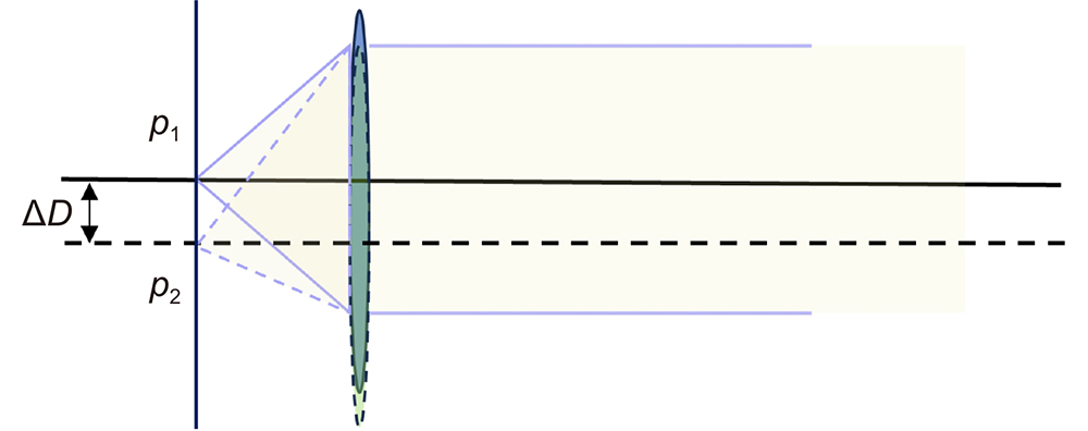
    Fig. 2. Schematic diagram of up-sampling based on micro-scanning
    Three ways of micro-scanning
    Fig. 3. Three ways of micro-scanning
    Schematic diagram of reconstruction based on micro-scanning imaging
    Fig. 4. Schematic diagram of reconstruction based on micro-scanning imaging
    Flow chart of our algorithm
    Fig. 5. Flow chart of our algorithm
    Schematic diagram of the experimental setup
    Fig. 6. Schematic diagram of the experimental setup
    Schematic diagram of selection module. Left: Image sequence; Right: An image grid with complete sub-pixel information
    Fig. 7. Schematic diagram of selection module. Left: Image sequence; Right: An image grid with complete sub-pixel information
    Four cases of displacement. (a) Four possible cases of pixel shift; (b) Four modes of integer pixel shift
    Fig. 8. Four cases of displacement. (a) Four possible cases of pixel shift; (b) Four modes of integer pixel shift
    Schematic diagrams of information extraction in four integer pixel shift cases
    Fig. 9. Schematic diagrams of information extraction in four integer pixel shift cases
    Schematic diagram of denoise module. (a) Schematic of matching same pixel of multiple images; (b) Pixel value and noise points (red circle) of same pixels
    Fig. 10. Schematic diagram of denoise module. (a) Schematic of matching same pixel of multiple images; (b) Pixel value and noise points (red circle) of same pixels
    Experiment sets of the active displacement imaging method
    Fig. 11. Experiment sets of the active displacement imaging method
    Camera position (red point)
    Fig. 12. Camera position (red point)
    Comparison result between ground truth and calculation. (a) Comparison result at 25 points; (b) Comparison of error at 25 points
    Fig. 13. Comparison result between ground truth and calculation. (a) Comparison result at 25 points; (b) Comparison of error at 25 points
    Super-resolution reconstruct results of different algorithms at scale of 4. (a) MFPOCS[20]; (b) ACNet[6]; (c) Ours
    Fig. 14. Super-resolution reconstruct results of different algorithms at scale of 4. (a) MFPOCS[20]; (b) ACNet[6]; (c) Ours
    MTF curves of different algorithms at different scales
    Fig. 15. MTF curves of different algorithms at different scales
    Original pictures and their ROI (red rectangle). (a) Simple image; (b) Complex image; (c) Panda image
    Fig. 16. Original pictures and their ROI (red rectangle). (a) Simple image; (b) Complex image; (c) Panda image
    Comparison of the traditional interpolation and our interpolation at 4 times. (a) Ground truth; (b) Ours; (c) Linear; (d) Bicubic
    Fig. 17. Comparison of the traditional interpolation and our interpolation at 4 times. (a) Ground truth; (b) Ours; (c) Linear; (d) Bicubic
    Super-resolution reconstruction results of simple image at different scales using the algorithms of MFPOCS[20](yellow rectangle), ACNet[6] (green rectangle) and ours (red rectangle)
    Fig. 18. Super-resolution reconstruction results of simple image at different scales using the algorithms of MFPOCS[20](yellow rectangle), ACNet[6] (green rectangle) and ours (red rectangle)
    Super-resolution reconstruction results of ROI of simple image at different scales using the algorithm of MFPOCS[20] (yellow rectangle), ACNet[6] (green rectangle) and ours (red rectangle)
    Fig. 19. Super-resolution reconstruction results of ROI of simple image at different scales using the algorithm of MFPOCS[20] (yellow rectangle), ACNet[6] (green rectangle) and ours (red rectangle)
    Super-resolution results of the complex image using the algorithms of MFPOCS[20] (yellow rectangle), ACNet[6] (green rectangle) and ours (red rectangle)
    Fig. 20. Super-resolution results of the complex image using the algorithms of MFPOCS[20] (yellow rectangle), ACNet[6] (green rectangle) and ours (red rectangle)
    Super-resolution reconstruction results of panda image at different scales using the algorithms of MFPOCS[20](yellow rectangle), ACNet[6](green rectangle) and ours (red rectangle)
    Fig. 21. Super-resolution reconstruction results of panda image at different scales using the algorithms of MFPOCS[20](yellow rectangle), ACNet[6](green rectangle) and ours (red rectangle)
    Super-resolution reconstruction results of the complex image at different scales using the algorithms of MFPOCS[20] (yellow rectangle), ACNet[6] (green rectangle) and ours (red rectangle)
    Fig. 22. Super-resolution reconstruction results of the complex image at different scales using the algorithms of MFPOCS[20] (yellow rectangle), ACNet[6] (green rectangle) and ours (red rectangle)
    Super-resolution reconstruction results of ROI of panda image at different scales using the algorithms of MFPOCS[20](yellow rectangle), ACNet[6] (green rectangle) and ours (red rectangle)
    Fig. 23. Super-resolution reconstruction results of ROI of panda image at different scales using the algorithms of MFPOCS[20](yellow rectangle), ACNet[6] (green rectangle) and ours (red rectangle)
    ImagesScale2345
    Simple imagePOCS[20]0.84930.80930.85680.8330
    ACNet[6]0.98760.97640.96230.9418
    Ours0.99210.96940.99490.9778
    Complex imageMFPOCS[20]0.68380.65390.68800.6714
    ACNet[6]0.94620.89260.80510.7358
    Ours0.95170.91830.95920.9250
    PandaMFPOCS[20]0.62630.61870.57480.5653
    ACNet[6]0.70460.67890.60140.5736
    Ours0.66960.62150.62550.6002
    Table 1. SSIM of three algorithms
    ImagesScale2345
    Simple imageMFPOCS[20]29.439026.423229.486826.4090
    ACNet[6]47.712543.635839.259336.5734
    Ours46.788345.572343.969939.1457
    Complex ImageMFPOCS[20]20.267220.129320.127020.1398
    ACNet[6]29.152127.745324.196121.9834
    Ours27.442429.539628.933226.6562
    PandaMFPOCS[20]24.072522.321520.437619.8857
    ACNet[6]25.761723.516919.504818.3985
    Ours24.003123.191521.975121.7718
    Table 2. PSNR of three algorithms
    ImagesScale2345
    Simple imageMFPOCS[20]314.7994211.4553131.7388105.3359
    ACNet [6]338.4507294.9276201.8644145.9228
    Ours320.5050265.3140215.9100184.1190
    Complex ImageMFPOCS[20]350.7845242.5359162.4356129.1925
    ACNet [6]471.1172395.2651275.1865216.5397
    Ours446.9067383.5727350.1874314.0308
    PandaMFPOCS[20]214.7590147.402691.817577.1331
    ACNet [5]271.9497263.0891191.2695163.3797
    Ours253.5610389.1927497.7272205.6040
    Table 3. Mean gradient of three algorithms
    Wenxue Zhang, Yihan Luo, Yaqing Liu, Shiye Xia, Kaiyuan Zhao. Image super-resolution reconstruction based on active displacement imaging[J]. Opto-Electronic Engineering, 2024, 51(1): 230290-1
    Download Citation