Individual Cow Recognition Based on Convolution Neural Network and Transfer Learning

Yongxin Xing; Biqiao Wu; Songping Wu; Tianyi Wang

doi:10.3788/LOP202158.1628002

Journals >Laser & Optoelectronics Progress >Volume 58 >Issue 16 >Page 1628002 > Article

Laser & Optoelectronics Progress
Vol. 58, Issue 16, 1628002 (2021)

Individual Cow Recognition Based on Convolution Neural Network and Transfer Learning

Yongxin Xing, Biqiao Wu, Songping Wu, and Tianyi Wang^*

Author Affiliations

College of Big Data and Information Engineering, Guizhou University, Guiyang 550025, Guizhou, China

show less

DOI: 10.3788/LOP202158.1628002 Cite this Article Set citation alerts

Yongxin Xing, Biqiao Wu, Songping Wu, Tianyi Wang. Individual Cow Recognition Based on Convolution Neural Network and Transfer Learning[J]. Laser & Optoelectronics Progress, 2021, 58(16): 1628002 Copy Citation Text

show less

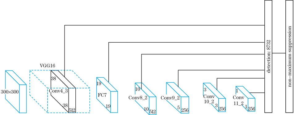
Fig. 1. SSD network structure

Download full size

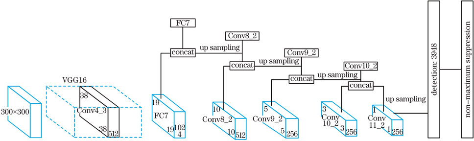
Fig. 2. Improvement of SSD network structure

Download full size

Fig. 3. Different fusion methods

Download full size

Fig. 4. Transfer learning process

Download full size

Fig. 5. Cow labeling pictures

Download full size

Fig. 6. P-R curves of different algorithms

Download full size

Fig. 7. Detection effect of improved SSD algorithm and SSD algorithm. (a) Improved SSD algorithm; (b) SSD algorithm

Download full size

Fig. 8. Loss curves of improved SSD algorithms under different training methods on training set

Download full size

Fig. 9. P-R curves of SSD algorithm with different training methods

Download full size

Fig. 10. P-R curves of improved SSD algorithm with different training methods

Download full size

Fig. 11. Detection effect of SSD algorithm with different training methods. (a) Transfer learning trains only the classification layer; (b) new study; (c) transfer learning trains all layers

Download full size

Fig. 12. Detection effect of improved SSD algorithm under different training methods. (a) Transfer learning trains all layers; (b) new study; (c) transfer learning trains only classification layer

Download full size

Feature map	M×N	K	Aspect ration	Number of candidate frames
Conv4_3	38×38	4	1,2	5776
FC7	19×19	6	1,2,3	2166
Conv8_2	10×10	6	1,2,3	600
Conv9_2	5×5	6	1,2,3	150
Conv10_2	3×3	4	1,2	36
Conv11_2	1×1	4	1,2	4

Table 1. Candidate box parameter setting of SSD algorithm

Upper sampling layer	Number of output channels		Kernel_size	Stride	Padding
Upper sampling layer	concat	add	Kernel_size	Stride	Padding
Conv11_2	256	256	3	3	Same
Conv10_2	256	256	3	1	Valid
Conv9_2	512	512	3	2	Same
Conv8_2	512	1024	10	1	Valid

Table 2. Parameter setting of upper sampling layer under different fusion modes

Feature map	M×N	K	Aspect_ration	Number of candidate frames
FC7	19×19	8	1,2,3,4	2888	3948
Conv8_2	10×10	8	1,2,3,4	800
Conv9_2	5×5	8	1,2,3,4	200
Conv10_2	3×3	6	1,2,3	54
Conv11_2	1×1	6	1,2,3	6

Table 3. Parameter setting of candidate frame of improved SSD algorithm

Experimental algorithm	Feature fusion	Fusion method	P_AP /%	Average detection time /ms
SSD			88.23	46.23
SSD	√	Add	88.11	51.52
SSD	√	Concat	90.58	54.04

Table 4. Experimental results on test sets of different fusion methods

Experimental algorithm	N_TP/N_FP/N_FN	P /%	R /%	P_AP/%	Average detection time /ms
SSD	454/12/60	97.42	88.32	88.23	46.23
Improved SSD	476/7/38	98.55	92.60	92.55	54.16

Table 5. Experimental results of SSD algorithm and improved SSD algorithm on test set

Experimental algorithm	Training method	N_TP/N_FP/N_FN	P /%	R /%	P_AP/%
SSD	New training	454/12/60	97.42	88.32	88.23
SSD	Transfer learning only trains classification layer	368/3/146	99.19	71.59	71.56
SSD	Transfer all levels of learning and training	477/8/37	98.35	92.80	92.69
Improved SSD	New training	476/7/38	98.55	92.60	92.55
Improved SSD	Transfer learning only trains classification layer	388/11/126	97.24	75.48	75.24
Improved SSD	Transfer all levels of learning and training	496/7/18	98.60	96.49	96.40

Table 6. Experimental results of different training methods on test set

Algorithm	20% of the training set	50% of the training set	80% of the training set	All training set
SSD	87.24	92.94	93.13	92.69
ImprovedSSD	91.73	95.10	95.66	96.40

Table 7. Influence of training set size of target domain on recognition accuracy after transfer learning

Algorithm	P_AP /%	Average detection time /ms
SSD	88.23	46.23
YOLOV2	85.26	20.49
YOLOV3	90.80	53.24
Method in Ref. [13]	85.46	19.64
Method in Ref. [14]	93.21	55.01
Method in this paper	96.40	54.16

Table 8. Average accuracy of different algorithms

Yongxin Xing, Biqiao Wu, Songping Wu, Tianyi Wang. Individual Cow Recognition Based on Convolution Neural Network and Transfer Learning[J]. Laser & Optoelectronics Progress, 2021, 58(16): 1628002

Download Citation

Set citation alerts for the article

Tools

Set citation alerts for the article

Save the article for my favorites

Paper Information