
A. S. Samsonov, I. Yu. Kostyukov, E. N. Nerush. Hydrodynamical model of QED cascade expansion in an extremely strong laser pulse[J]. Matter and Radiation at Extremes, 2021, 6(3): 034401
- Matter and Radiation at Extremes
- Vol. 6, Issue 3, 034401 (2021)
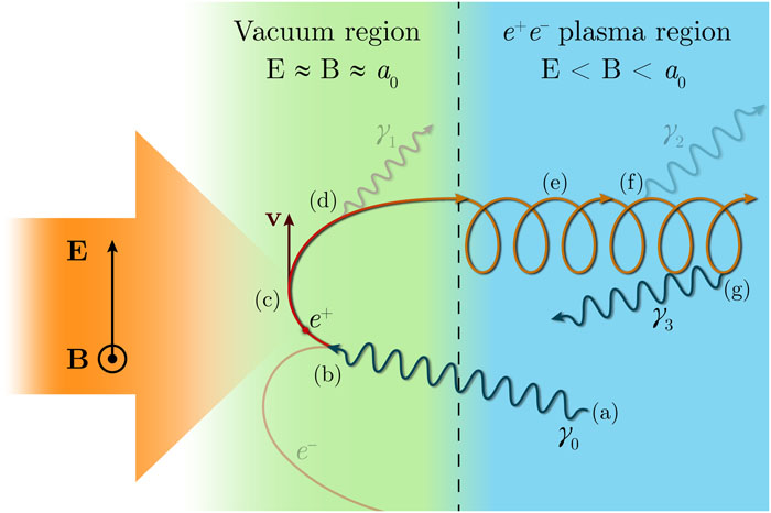
Fig. 1. Core mechanism of cascade self-sustenance. (a), (f), and (g) Emission of a gamma quantum in the plasma region or the involved gamma quantum. (b) Decay of the involved gamma quantum in the vacuum region. (c) Positron and electron acceleration in the plane wave. (d) Emission of the gamma quantum in the vacuum region or the decoupled gamma quantum. (e) Helical motion of the positron in the plasma region.
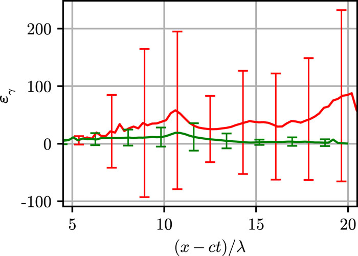
Fig. 2. Mean energy ɛ γ of gamma quanta located in the vicinity of the x coordinate calculated from all the particles (red line) and from the particles with velocity along the x axis less than 0.5, which supposedly include only the involved gamma quanta (green line). The error bars depict the standard deviation. The data are taken from the results of the PIC simulation for the time instant ct /λ = 18. The simulation parameters are discussed in Sec. III . The initial conditions are the same as in Fig. 6 .
Fig. 3. Validation of the approximation used for describing angular distribution of the particles. (a) and (c) Angular distributions of gamma quanta (a) and pairs (c) located in the vicinity of the coordinate x (color map) and the mean longitudinal velocity calculated from the distribution (black line) computed from the results of the QED-PIC simulation. (b) and (d) Angular distributions of gamma quanta (b) and pairs (d) calculated from the mean velocity using the expression (25) .
Fig. 4. Validation of the approximations used in the model. (a) Value of the product j · E computed from Eq. (35) and computed directly from the results of the QED-PIC simulations. (b) Mean longitudinal velocity of pairs computed from Eq. (49) and computed directly from the results of the QED-PIC simulations. (c) Distributions of electric field, magnetic field, and plasma density. Each plot is computed from the data averaged over a ±2λ vicinity around the laser pulse axis in the yz plane.
Fig. 5. Relation between the velocity vector and the magnetic field vector in the reference frame K ′ moving along the x axis with velocity v x = E /B .
Fig. 6. Comparison between the solution of Eqs. (52) –(57) [(a), (c), and (e)] and the results of the QED-PIC simulations [(b), (d), and (f)] for laser amplitude a 0 = 2500 and n γ ,0 = 0.5a 0n cr. (a) and (b) Distributions of gamma-quantum density n γ , electromagnetic energy density (E 2 + B 2)/2, and plasma density n p at different time instants. Note that the scale of the vertical axis is linear in the range [0, 1] and logarithmic in the range [1, +∞]. (c) and (d) Energy balance: total energy of pairs Σp and of gamma quanta Σγ and electromagnetic energy ΣEM, all normalized to the initial total energy of the system Σtot. The velocity of the plasma boundary v fr is also plotted. (e) and (f) Distribution of pairs in the xt plane and the position of the plasma boundary x fr. The numerical values of the fitting parameters used in the model solution are ν = 0.32 and μ = 10.
Fig. 7. Same as Fig. 6 , but for a 0 = 1500 and n γ ,0 = a 0n cr. The values of the fitting parameters are ν = 0.35 and μ = 10.
Fig. 8. Same as Fig. 6 , but for a 0 = 1000 and n γ ,0 = a 0n cr. The values of the fitting parameters are ν = 0.35 and μ = 10.
Fig. 9. Velocity of the cascade front observed in the model solution (green line) and obtained from the simplified model developed in Ref. 37 (red line) calculated from the mean velocity of the particles located at a depth of 2λ behind the cascade front.
Fig. 10. Validation of the approximations used to describe the energy gain due to acceleration and the energy loss due to gamma-quantum emission by a single particle in a plane wave for a 0 = 2500, p 0 = 500, and θ = π . The solid lines correspond to the numerical solution of Eqs. (A33) –(A35) and the dashed lines to the approximations (A40) and (A41) , where μ = ct /3λ .
Fig. 11. Longitudinal velocity v x computed by numerical solution of Eqs. (B11) and (B12) (green line) and from the approximate expression (B17) (red line) for the plasma density in the form of an inhomogeneous slab (black line). In (a), the scale of inhomogeneity is smaller than the wavelength, and hence the WKB approximation is valid, while in (b), the scale of inhomogeneity is larger than the wavelength.


Set citation alerts for the article
Please enter your email address

© Copyright 2018-2021 | Chinese Laser Press. All Rights Reserved 沪ICP备15018463号-20