
Ping Yin, Aijun Xu, Jianxin Yin. Generating Disparity Image of Standing Trees Based on Improved SGM[J]. Laser & Optoelectronics Progress, 2022, 59(18): 1815017
- Laser & Optoelectronics Progress
- Vol. 59, Issue 18, 1815017 (2022)
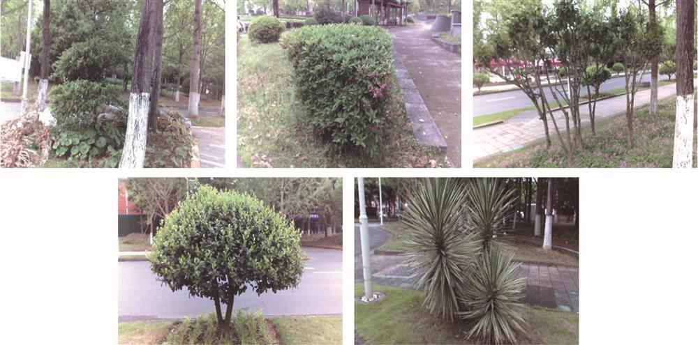
Fig. 1. Five species of tree
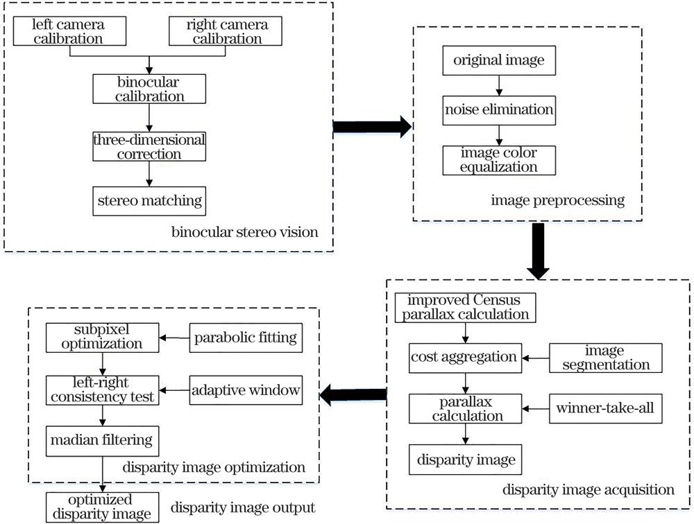
Fig. 2. Flowchart of tree disparity image generation method
Fig. 3. Median calculation
Fig. 4. Cost aggregation. (a) Minimum path cost; (b) 8-path aggregation
Fig. 5. Schematic of winner-take-all algorithm
Fig. 6. Correction results of tree image. (a) Before correction; (b) after correction
Fig. 7. Histogram equalization results before and after preprocessing. (a) Tree left image; (b) tree right image; (c) tree left image after preprocessing; (d) tree right image after preprocessing
Fig. 8. Disparity images generated by different algorithms. (a) SGBM algorithm; (b) BM algorithm; (c) SGM algorithm; (d) proposed algorithm
Fig. 9. Comparison between the disparity image generated by the proposed algorithm and the real disparity image. (a) Original left image; (b) real disparity image; (c) disparity image generated by the proposed algorithm
|
Table 1. Algorithm parameters in this paper
| ||||||||||||||||||
Table 2. Calibration results of binocular camera
|
Table 3. Matching cost test result
|
Table 4. False match rate of different algorithms on Middlebury standard dataset

Set citation alerts for the article
Please enter your email address
© Copyright 2018-2021 | Chinese Laser Press. All Rights Reserved 沪ICP备15018463号-20