Hyperspectral Image Classification Based on Edge-Preserving Filter and Deep Residual Network

Lü Huanhuan; Zhuolu Wang; Hui Zhang

doi:10.3788/LOP202259.1611005

Journals >Laser & Optoelectronics Progress >Volume 59 >Issue 16 >Page 1611005 > Article

Laser & Optoelectronics Progress
Vol. 59, Issue 16, 1611005 (2022)

Hyperspectral Image Classification Based on Edge-Preserving Filter and Deep Residual Network

Lü Huanhuan^1、2, Zhuolu Wang¹, and Hui Zhang^2、*

Author Affiliations

¹School of Software, Liaoning Technical University, Huludao 125105, Liaoning , China

²School of Information Engineering, Huzhou University, Huzhou 313000, Zhejiang , China

show less

DOI: 10.3788/LOP202259.1611005 Cite this Article Set citation alerts

Lü Huanhuan, Zhuolu Wang, Hui Zhang. Hyperspectral Image Classification Based on Edge-Preserving Filter and Deep Residual Network[J]. Laser & Optoelectronics Progress, 2022, 59(16): 1611005 Copy Citation Text

show less

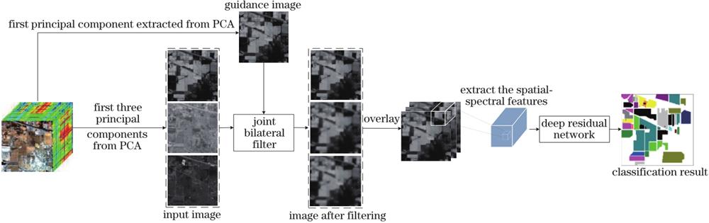
Fig. 1. Overall flow of the proposed method

Download full size

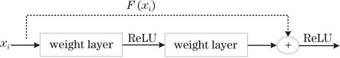
Fig. 2. Structure diagram of residual element

Download full size

Fig. 3. Model structure of depth residual network

Download full size

Fig. 4. Indian Pines dataset. (a) False color image;(b) real ground data

Download full size

Fig. 5. Pavia University dataset. (a) False color image;(b) real ground data

Download full size

Fig. 6. Classification accuracy of different dropout values. (a) Indian Pines; (b) Pavia University

Download full size

Fig. 7. Loss function and overall classification accuracy of different epoch values. (a) Indian Pines; (b) Pavia University

Download full size

Fig. 8. Classification accuracy of different

η

values. (a) Indian Pines; (b) Pavia University

Download full size

Fig. 9. Overall classification accuracy of different

δ_{c}

values and

δ_{s}

values. (a) Indian Pines; (b) Pavia University

Download full size

Fig. 10. Classification results of different algorithms in Indian Pines dataset

Download full size

Fig. 11. Partial enlargement comparison of classification results of Indian Pines dataset

Download full size

Fig. 12. Classification results of different algorithms in Pavia University dataset

Download full size

Fig. 13. Partial enlargement comparison of classification results of Pavia University dataset

Download full size

Input layer	Layer	Feature map size	Params
Total number of parameters		1276592
	Input	9，9，3	0
Input	C1	7，7，16	448
C1	C2	7，7，32	4640
C2	C3	7，7，32	9248
C1	R1	7，7，32	4640
C3、R1	Add1	7，7，32	0
Add1	Activation1	7，7，32	0
Activation1	C4	7，7，64	18496
C4	C5	7，7，64	36928
C1	R2	7，7，64	9280
Activation1	R4	7，7，64	18496
C5、R2、R4	Add2	7，7，64	0
Add2	Activation2	7，7，64	0
Activation2	C6	7，7，128	73856
C6	C7	7，7，128	147584
C1	R3	7，7，128	18560
Add1	R5	7，7，128	36992
Add2	R6	7，7，128	73856
C7、R3、R5、R6	Add3	7，7，128	0
Add3	Activation3	7，7，128	0
Activation3	P1	5，5，128	0
P1	Flatten1	3200	0
Flatten1	FC	256	819456
FC	Dropout	256	0
Dropout	Softmax	16	4112

Table 1. Feature map size and parameter quantities of depth residual network

Number of convolution kernels	Indian Pines		Pavia University
Number of convolution kernels	OA /%	Kappa /%	OA /%	Kappa /%
8	88.54	86.94	90.34	88.92
16	92.16	91.06	92.53	91.57
32	91.29	90.08	93.53	92.98
64	90.75	89.62	91.01	89.92

Table 2. Classification accuracy corresponding to different numbers of convolution kernels

Class	SP-SVM	2DCNN	Res-3DCNN	S2FEF-CNN	LBP-1DCNN	Res-2DCNN	JBF-2DCNN	JBF-Res- 2DCNN
Alfalfa	60.86	81.81	71.42	82.60	88.37	100.00	97.43	100.00
Corn-notill	76.43	78.35	91.25	90.98	94.88	98.40	98.75	96.87
Corn-min	72.89	84.26	89.79	92.65	95.29	95.04	96.58	97.36
Corn	57.56	64.95	82.43	89.04	89.37	91.54	98.03	100.00
Grass/pasture	90.11	90.42	92.80	91.87	92.93	98.57	95.55	99.08
Grass/trees	87.84	94.94	93.40	98.94	99.24	96.60	99.84	100.00
Grass-mowed	87.50	100.00	88.00	77.41	75.00	90.00	96.00	100.00
Hay-windrowed	93.18	96.57	94.05	99.53	100.00	100.00	100.00	100.00
Oats	50.00	87.50	90.90	50.00	52.17	43.47	87.50	90.00
Soybeans-notill	75.08	79.77	88.53	91.06	93.20	93.87	96.50	98.06
Soybeans-min	78.52	81.88	94.96	94.57	96.76	97.47	96.39	99.77
Soybeans-clean	83.40	81.97	88.69	91.49	92.91	96.24	97.70	97.55
Wheat	97.29	94.32	100.00	100.00	100.00	100.00	100.00	100.00
Woods	93.11	93.37	98.57	99.29	99.11	98.94	99.38	99.91
Bldg-grass-drives	77.94	75.95	89.94	93.87	94.66	96.50	95.22	99.71
Stone-steel-towes	98.57	100.00	98.61	96.92	95.52	100.00	100.00	100.00
OA	81.56	84.71	92.78	94.17	95.83	96.92	97.62	98.87
AA	80.02	86.63	90.83	90.01	91.21	93.54	97.18	98.64
Kappa	78.90	82.53	91.77	93.35	95.25	96.60	97.28	98.71

Table 3. Classification results of different algorithms in the Indian Pines dataset

Class	SP-SVM	2DCNN	Res-3DCNN	S2FEF-CNN	LBP-1DCNN	Res-2DCNN	JBF-2DCNN	JBF-Res-2DCNN
Asphalt	81.44	89.37	93.31	95.09	96.08	97.95	98.20	99.38
Meadows	90.26	91.67	95.12	97.83	99.23	98.36	99.78	99.92
Gravel	82.63	83.31	80.16	93.27	94.96	91.80	92.18	96.32
Trees	95.65	96.74	99.91	99.24	97.74	98.18	96.78	99.45
Painted metalsheets	99.15	99.15	91.76	99.23	100.00	97.09	100.00	98.02
Bare soil	94.11	94.23	95.08	97.74	97.41	95.74	99.59	100.00
Bitumen	94.77	87.69	83.94	83.96	85.22	98.73	95.30	98.84
Self-blocking bricks	79.26	80.90	86.07	86.52	88.15	90.23	93.54	97.67
Shadows	100.00	100.00	100.00	100.00	100.00	100.00	100.00	100.00
OA	88.58	90.86	93.28	95.85	96.78	97.14	98.26	99.35
AA	90.81	91.45	91.71	94.76	95.42	95.96	97.26	98.84
Kappa	84.53	87.69	91.01	94.48	95.73	96.48	97.69	99.13

Table 4. Classification results of different algorithms in Pavia University dataset

Dataset	Parameter	Algorithm
Dataset	Parameter	SP-SVM	Res-3DCNN	S2FEF-CNN	LBP-1DCNN	JBF-Res-2DCNN
Indian Pines	Training time	18.64	1507.28	1430.21	890.49	1293.52
Indian Pines	Test time	0.75	5.06	3.91	2.78	3.04
Pavia University	Training time	10.31	1002.79	921.52	629.46	862.95
Pavia University	Test time	1.42	8.35	7.28	5.05	5.93

Table 5. Training time and test time of different algorithms

Lü Huanhuan, Zhuolu Wang, Hui Zhang. Hyperspectral Image Classification Based on Edge-Preserving Filter and Deep Residual Network[J]. Laser & Optoelectronics Progress, 2022, 59(16): 1611005

Download Citation

Set citation alerts for the article

Tools

Set citation alerts for the article

Save the article for my favorites

Paper Information