
Luke Horstman, Ning Hsu, James Hendrie, David Smith, Jean-Claude Diels. Exceptional points and the ring laser gyroscope[J]. Photonics Research, 2020, 8(3): 252
- Photonics Research
- Vol. 8, Issue 3, 252 (2020)
![Sketches of bidirectional ML gyro configurations (left) and their corresponding beat-note responses (right). The × corresponds to a pulse crossing that does not introduce phase coupling. G is the gain, and Δϕ=Δ/τrt is the differential round-trip phase shift. Note that the time unit in Eq. (1) has been normalized to τrt. (a) Linear (i.e., no dead band) response. (b) When a scattering interface is placed at the crossing point, a square-root (i.e., dead band) response is observed (data from Ref. [21]).](/richHtml/prj/2020/8/3/03000252/img_001.jpg)
Fig. 1. Sketches of bidirectional ML gyro configurations (left) and their corresponding beat-note responses (right). The × G is the gain, and Δ ϕ = Δ / τ r t 1 ) has been normalized to τ r t
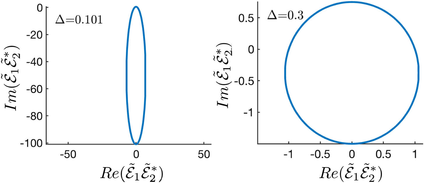
Fig. 2. Polar plots of the imaginary versus real part of the beat field near (left) and far (right) from the EP (dead band). Near the EP the beat note stems from amplitude modulation, while far from the EP it is caused by pure phase modulation.
Fig. 3. Beat-signal spectrum from a numerical solution of Eq. (1 ) (top), and experimentally measured beat-note signal (bottom) showing the clustering of frequency harmonics near the dead band (left) and their absence for larger Δ
Fig. 4. Beat-signal spectrum from a numerical solution of Eq. (1 ) showing the clustering of harmonics near the EP (dead band).
Fig. 5. Gyro beat-note response curve changes with κ ˜ s 1 ) with κ ˜ = 0.05 s = 0 s = 0.03 s = 0.05 s = 0.06 κ ˜ = 0 s = 0.05 2 Δ ω 5 ). When saturable gain is included, the green circles shift to the positions of the cyan crosses because the COG (rather than the most prevalent peak) of the spectrum must be used. An example of data matching the κ ˜ = 0
Fig. 6. Numerical solution (blue circles) to Eq. (1 ) and analytic prediction (red dashes) of Eq. (6 ) showing an EP at Δ = 0 κ ˜ = 0.05 α ^ 1 = 0.051 α L = 0 β = 1 γ = 0 α 2 = − | κ ˜ | = − 0.05 Δ Δ = 0 Visualization 1 for Δ = 0.01

Set citation alerts for the article
Please enter your email address
© Copyright 2018-2021 | Chinese Laser Press. All Rights Reserved 沪ICP备15018463号-20