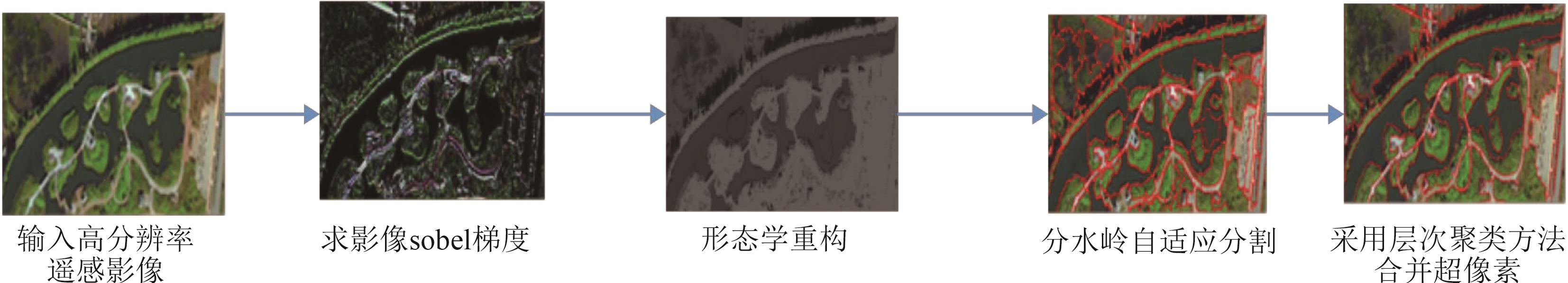
Fig. 1. Flow chart of remote sensing image segmentation

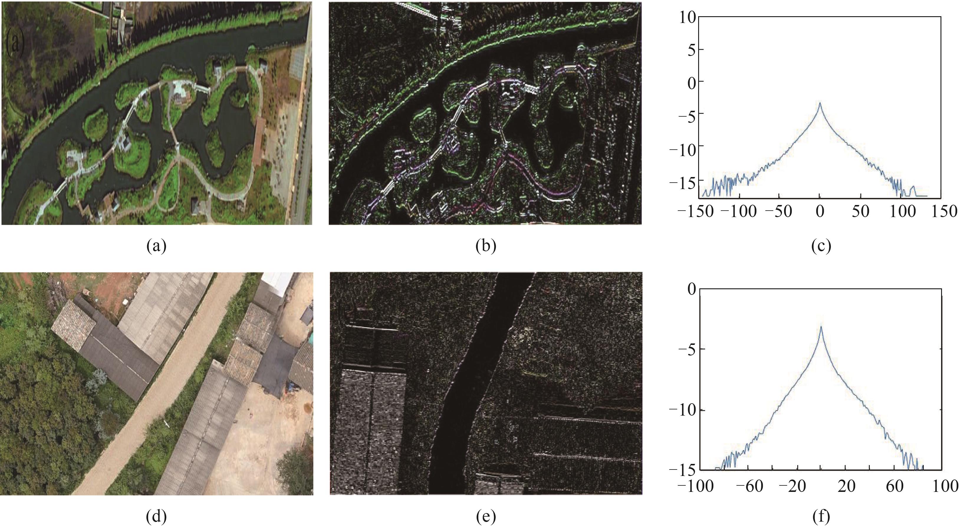
Fig. 2. Gradient distribution of experimental images（a） remote sensing image, （b） sobel gradient image, （c） gradient distribution, （d） remote sensing image, （e） sobel gradient image, （f） gradient distribution

Fig. 3. Segmentation results using AMR-WT by changing the value of s and m（a） s = 1, m = 1; （b） s = 2, m = 1; （c） s = 3, m = 1; （d） s = 4, m = 1; （e） S₁s = 1, m =1; （f） S₂s = 1, m = 6; （g） s = 1, m = 12; （h） s = 1, m = 20

Fig. 4. Simulation graph of clustering（a）clustering simulation, （b）segmentation results, （c）clustering simulation, （d）segmentation results

Fig. 5. Test data sets （a） S₁ imag, （b） S₂ image, （c） S₃ image, （d） S₄ image, （e） S₁ image, （f） S₂ reference image, （g） S₃ reference image, （h） S₄ reference image

Fig. 6. Experimental results of over-segmentation（a） S₁ proposed superpixel algorithm, （b） S₁ SLIC algorithm, （c） S₁ LSC algorithm, （d） S₁ Meanshift algorithm, （e） S₂ proposed superpixel algorithm, （f） S₂ SLIC algorithm, （g） S2 LSC algorithm, （h） S₂ MeanShift algorithm, （i） S₃ proposed superpixel algorithm, （j） S₃ SLIC algorithm, （k） S₃ LSC algorithm, （l） S3 Meanshift algorithm, （m） S₄ proposed superpixel algorithm, （n） S₄ SLIC algorithm, （o） S₄ LSC algorithm, （p） S₄ MeanShift algorithm

Fig. 7. The time of over-segmentation

Fig. 8. Segmentation results of S₁ and S₂ （a） S1 FNEA 50, （b） S₁ FNEA 100, （c） S₁ SH method, （d） result of S₁ by proposed method, （e） S₂ FNEA 50, （f） S₄ FNEA 100, （g） S₂ SH method, （h） result of S₂ by proposed method

Fig. 9. Segmentation results of Test1

Fig. 10. Segmentation results of S₃ and S₄（a） S₃ FNEA 50, （b） S₃ FNEA 100, （c） S₃ SH method, （d） S₃ result by proposed method, （e） S₄ FNEA 50, （f） S₄ FNEA 100, （g） S₄ SH method, （h） S₄ result by proposed method

Fig. 11. Segmentation results of Test2

Table 1. Information of segmentation data sets