Abstract
The previous methods to measure flow speed by photoacoustic microscopy solely focused on either the transverse or the axial flow component, which did not reflect absolute flow speed. Here, we present absolute flow speed maps by combining Doppler bandwidth broadening with volumetric photoacoustic microscopy. Photoacoustic Doppler bandwidth broadening and photoacoustic tomographic images were applied to measure the transverse flow component and the Doppler angle, respectively. Phantom experiments quantitatively demonstrated that ranges of 55° to 90° Doppler angle and 0.5 to 10 mm/s flow speed can be measured. This tomography-assisted method provides the foundation for further measurement in vivo.Photoacoustic (PA) imaging (PAI) combines the advantages of pure optical imaging and ultrasonic imaging with high spatial resolution and high image contrast[1–5]. These merits help to open up broad implementations such as PA microscopy (PAM)[6,7], tomography[8], endoscopy[9,10], and intravascular imaging[11]. PAM is a new technology for measuring flow speed. It measures flow speed by extracting Doppler shift, transit time, tracking density, and encoding amplitude of light-absorbed media[12]. Unlike Doppler ultrasound technology, which suffers from poor spatial resolution in measuring relatively low-speed flow in microcirculation networks, optical-resolution PAM (OR-PAM) provides high sensitivity to detect microcirculation based on focused laser beams[13]. Previous researches[14–17] have shown a variety of estimation methods for either axial or transverse flow components. However, the flow could orient a variety of directions and angles. Therefore it is inaccurate to analyze the absolute flow speed by measuring only one flow component. It was generally thought that if the absolute flow speed is to be measured, it is needful to measure both axial and transverse flow components or analyze the flow speed by other complicated calculations[18–20]. Both the axial and transverse flow components were considered to estimate the absolute flow speed by Yao et al.[18], with the axial component being obtained by using the phase shift between consecutive Hilbert-transformed pairs of A-lines, and the transverse component being quantified from bandwidth broadening via Fourier transformation of sequential A-lines. However, obtaining the absolute flow speed by calculating two velocity components is obviously more complicated than that by calculating only one component. To obtain the Doppler angle, Song et al.[19] extracted the distance between the transducer and three adjacent scanning points along the flow and repeatedly applied the Law of Cosines, increasing the computational complexity and calculating load. Moreover, time shift between two consecutive PA waves needs to be calculated to measure flow velocity along the ultrasonic detection axis at the same scanning point, resulting in increased complexity.
In this Letter, to calculate the absolute flow speed, we proposed a method that combines the transverse flow component by using PA Doppler bandwidth broadening and Doppler angle by superimposing the PA tomograms into three-dimensional images. This method, compared with combination of two flow components, can reduce the complexity of the calculation and system without increasing the number of transducers. The abilities of the method to measure flow speed and Doppler angle were verified in microtube phantoms filled with light-absorbed flowing microspheres and rabbit blood.
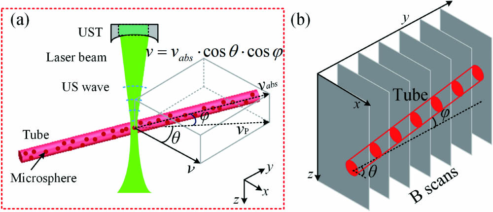
Figures 1(a) and 1(b) illustrate the methods to measure absolute flow speed and Doppler angle. To measure the transverse flow component, gaining enlightenment from real-time ultrasonic Doppler blood-flow imaging[21], the PA broadening bandwidth, , was statistically obtained. The PA A-line signal was passed through a digital bandpass filter prior to the estimation of . Then, the standard deviation of complex function sequential A-lines signals is used to calculate by[22]where is the calculated standard deviation, denotes the Hilbert transformation of the th A-line signal, is the complex conjugate of , is the time interval between sequential A-scans, is the number of all A-lines, and is a calibration factor that is determined by the focusing mechanism of the system. Then, the transverse flow component can be calculated as[22,23]where is the speed of sound in water, is the central frequency of the PA signal, is the effective aperture of the objective lens, and is the Doppler angle.
Sign up for Chinese Optics Letters TOC. Get the latest issue of Chinese Optics Letters delivered right to you!Sign up now

Figure 1.(a) Beam geometry of PA flow speed measurement. US, ultrasound; UST, ultrasound transducer. (b) Geometry of the Doppler angle by superimposing of a set of PA images to form volumetric images.
To obtain the Doppler angle, dozens of PA tomographic images (B-scans) were superimposed to form a volumetric vascular structure, as shown in Fig. 1(b). Then, the angle between the tube and its bottom-projected line and the angle between the B-scan base level and the tube-projected line can be measured. The absolute flow speed is derived [Fig. 1(a)] as
The schematic setup is shown in Fig. 2(a), where the PAM system employs a frequency-doubled neodymium-doped yttrium aluminum garnet (Nd:YAG) laser (Model DTL-314QT, Laser-export) for PA irradiation at a single optical wavelength of 532 nm and pulse duration of 10 ns. The laser pulse repetition rate (PRR) was controlled at 5 kHz. The laser beam was focused onto the sample through an objective lens () with large focal distance after passing through a beam expanding and collimating system. The pulse energy after the objective lens is measured to be ∼50 nJ. A custom-made hollow focused ultrasonic transducer (focus diameter of 16.3 mm and central frequency of 10 MHz) was aligned coaxially with the objective lens to maximize the sensitivity, and the detected PA signal was amplified by a low-noise amplifier (LNA, gain of 50 dB, Rfbay). The data is processed by Matlab in a computer.
Figure 2.(a) Schematic of the photoacoustic imaging system. BS, beam splitter; DAQ, data acquisition card; L1 and L2, lenses; M1 and M2, mirrors; Ob, objective; PD, photodiode; PH, pinhole; WT, water tank. (b) Original PA signal along the dashed line of the inserted photograph of a blade, and its line spread function whose full width at half-maximum was measured to be ∼7 μm. (c) The lateral resolution versus the axial distance. (d) Pulse-echo response of the ultrasonic transducer at the focus. (e) The signal-to-noise ratio (SNR) versus the axial distance.
Figure 2(b) indicates the full width at half-maximum (FWHM) of the line-spread function (LSF) defining the lateral resolution of the PAI system, which is ∼7 μm, with an inserted picture of the maximum amplitude projection (MAP) image of a sharp-edged surgical blade. The measured resolution is larger than the theoretical resolution (∼3 μm) because the NA of the laser beam was reduced when it was in water. The concentration of light-absorbed articles ought to be appropriate, and the optical focus of OR-PAM or the acoustic focus of acoustic resolution PAM ought to be tight enough, with the optimal diameter to be around one red blood cell (RBC) of ∼6 μm diameter to differentiate the signal fluctuation resulting from RBCs or other light-absorbed article flow[17]. Tissue-induced light scattering and resolution deteriorating could be mitigated by extending the depth-of-field, such as focus-adjusting technology[24–26], Bessel beam[27], synthetic aperture focus technology for optical beams[28], and transducer-array-based super-fast imaging[29]. Figure 2(c) presents the lateral resolution versus the axial distance, which demonstrates that the lateral resolution still remains no more than two RBCs (∼12 μm) in hundreds-of-micrometer depths. Figure 2(d) shows the pulse-echo response of the transducer at the focus (black line), and the red line is the Hilbert-transformed envelope of a typical signal. The axial resolution of the PAI system can be taken as FWHM of the envelope, which is measured to be ∼126.6 μm. Figure 2(e) illustrates the signal-to-noise ratio (SNR) versus the axial distance, whose result corresponds well with the lateral resolution.
We validated the correlation-based transverse flow component measurement in a blood-mimicking phantom experiment. Specifically, a syringe pump (Linger Pump Inc.) was used to drive light-absorbed microspheres (mean diameter: 6 μm, Polysciences Inc.) through a plastic tube with inner and outer diameters of ∼250 μm and ∼350 μm, respectively. The step sizes of the bi-directional scanning were set to be ∼3 μm, which are no more than half of the lateral resolution to achieve optimum image quality[30]. Figure 3(a) shows a representative PA MAP image along the plane across a randomly chosen cross section of the tube, and a typical transverse flow image is shown in Fig. 3(b). It can be seen that the flow speeds decrease from the center to the edge, which tallies with the feature of laminar flow.
Figure 3.Photoacoustic (a) maximum amplitude projection and (b) transverse flow of a phantom. (c) Measured bandwidth with the Doppler angle of 90° versus preset speed with consecutive A-lines of 2/4/6/8/10. Measured bw., measured bandwidth. (d) Measured maximum non-saturated bandwidth with the Doppler angle of 90° versus consecutive A-lines of 2 to 30. Max. ms., maximum measured speed; Num. of A-line for corr. cal., number of A-line for correlation calculation. (e) Ten representative consecutive A-lines.
At a fixed position of the center of the tube, 3000 sequential A-lines were acquired, filtered, and grouped every 30 lines. The number of consecutive A-lines chosen from each group to conduct transverse flow speed calculation, by Eqs. (1) and (2), was set from 2 to 30 with increments of one [Fig. 3(e) shows a group of representatives], since in previously reported studies[17,18], this number was usually set to be eight, without explanation or further research. Here, how many consecutive A-lines being selected is better for calculation has been studied. Five cases with 2/4/6/8/10 sequential A-lines are shown in Fig. 3(c), from which it can be seen that the maximum measurable non-saturated broadening bandwidth increases as the number of A-lines raises. Specifically, when 2 A-lines were selected, the maximum measurable non-saturated broadening bandwidth was calculated to be ∼40 Hz at 2.5 mm/s, and four A-lines to be ∼50 Hz at 3 mm/s, six A-lines to be ∼70 Hz at 6 mm/s, eight A-lines to be ∼90 Hz at 10 mm/s, and 10 A-lines to be ∼100 Hz at 10.5 mm/s. Further, the corresponding relationship was applied to all cases from 2 to 30 A-lines, deriving a fitted profile shown in Fig. 3(d), which illustrates that the maximum measurable speed by our system is higher than 10 mm/s with 10 A-lines being calculated and nearly remain steady when beyond 10 A-lines. It is necessary to point out that it is the Brownian motion of microspheres that results in non-zero broadening bandwidth when speed was set at 0 mm/s[23,31,32].
It is worthy of attention that, as particles flow quicker through the focus, the transit time becomes shorter, and the bandwidth, which is its inverse, broadens by[23]where is the flow speed, is the speed of sound, is the Doppler angle, and , , and are the center frequency, the diameter, and the focus length of the ultrasonic transducer, respectively. The Doppler bandwidth is proportional to the transverse flow speed and is maximized when the Doppler angle is 90°.
Figure 4 shows the results of measuring Doppler angle. The angle between the axis of the ultrasound transducer and the microtube centerline was set to be 55° to 90° with an increment of 5°. It should be noted that this range of measured Doppler angle was confined by the coaxially light–sound geometric structure but would not affect its practicability. Figure 4(a) illustrates the approach of measuring the Doppler angle by measuring the projected angles in the and planes, with five groups of representative angles (55°, 65°, 75°, 85°, and 90°) being shown. According to solid geometry, the angle between two straight lines is equal to the angle between the planes in which the straight lines are separately located. The Doppler angle can thus be derived from the projected angle in the plane, as shown in the second row of Fig. 4(a). Figure 4(b) shows the measured angles versus preset values, coinciding with each other well. Figure 4(c) shows the fitted distributions of flow speeds across the tube along the axis, which demonstrates that the maximum speed decreases as the Doppler angle decreases, being consistent with the theory. Further, hundreds of A-lines were acquired at the center of the tube with the same speed but different angles, to testify to transverse flow speed versus preset angle, whose result is shown in Fig. 4(d). The fitted line of the experimental statistics accords well with theory that the relationship between the transverse flow speed and the preset angle satisfies the trigonometric function.
Figure 4.Measurement of Doppler angle. (a) Illustration of Doppler angles (55°, 65°, 75°, 85°, and 90°) derived from volumetric image. (b) Comparison of preset and measured Doppler angles. Meas. angle, measured angle. (c) Measured transverse speed profiles along the cross section of the tube with different angles. (d) Measured transverse speed profiles at the center of the tube with different angles.
To testify to the ability of this method to distinguish artery and vein phantoms, whose outer and inner diameters were ∼350 μm and ∼250 μm, respectively, the tubes were fixed in a water tank and injected with rabbit blood at the speed of one tube being set faster than that of the other. A volumetric dataset was acquired for structural and flow imaging. Figures 5(a) and 5(b) denote the volumetric image and section of the structure profile, respectively. The MAP image shows inconspicuous difference between the two tubes, while in the speed image, as Fig. 5(c) illustrates, the slower flow areas appear slightly darker than the faster flow regions. Further, the Doppler angles of the two tubes were measured, as illustrated in Fig. 5(e). Figure 5(d) shows the image of absolute speed of the two tubes, which was calculated by combining the transverse flows and Doppler angles mentioned above within the tube-based area, and Fig. 5(f) shows the comparison between the profiles of transverse and absolute speeds. It can be seen that the transverse flow speed was measured to be obviously smaller than the absolute flow speed because of the former’s intrinsically neglecting the Doppler angle.
Figure 5.Results of artery and vein phantom experiments. (a) Volumetric and (b) MAP images of two tubes. (c) Transverse flow speed image of the two tubes. (d) Absolute speed mapping of the two tubes, which was calculated by combining transverse flows and Doppler angles within the tube-based area. (e) Doppler angles of the two tubes. (f) Profiles of transverse (blue curve) and absolute (red curve) speed of the dashed line in (c) and (d).
Theoretically, the maximum measurable speed is limited by laser repetition rate and light beam focus diameter. Meanwhile, many factors, such as electronic noise and ambient vibrations, which affect the SNR, plus acquisition time, decide the minimum measurable speed and the speed resolution, which were measured to be around 0.5 mm/s in this work and can be improved by clutter filtering. Increasing the repetition rate of the excitation and the size of the focal spot could enhance the value of the upper measurable speed, but both accuracy and resolution also decrease[17,22].
Although many previous PA methods to measure flow speeds provide the flow direction information, which the PA Doppler bandwidth broadening measurement method loses due to its symmetry[22], they solely focused on one flow component, resulting in an inaccurate absolute speed measurement, and multi-transducers need to be employed to collect bi-component signal, increasing system complexity, or they applied M-scan along the flow direction, limiting their application. Several emerging methods to estimate blood-flow speed, such as a dual-pulse method based on the Grueneisen relaxation effect[33] and a parallel computation design based on graphics processing unit[34], offered time-saving acquisition and wide measurable speed range, which means they may play a better role in measuring flow components.
In summary, the feasibility of combining Doppler angle and bandwidth broadening measurements to calculate absolute flow speed was demonstrated in vessel-mimicking phantoms. The advantage of this method is simplicity: only one ultrasound transducer is enough to obtain absolute flow speed. Admittedly, under normal physiological conditions, effects of breath, heartbeat, and strong clutters from tissue are inevitable, which indicates that clutter rejection should be added in our future in vivo research lists; yet the unevenness of biological skin remains another challenge, which induces significant deterioration of resolution and should be considered to be mitigated by methods mentioned previously like Bessel beam synthetic aperture focus technology, etc. Manual measurement of the Doppler angle will be replaced by machine learning or other image processing technologies to realize angle auto-measurement from tomographic images.
References
[1] P. Beard. Interface Focus, 1, 602(2011).
[2] C. Li, L. V. Wang. Phys. Med. Biol., 54, R59(2009).
[3] M. Omar, J. Aguirre, V. Ntziachristos. Nat. Biomed. Eng., 3, 354(2019).
[4] K. Xia, X. Zhai, Z. Xie, K. Zhou, Y. Feng, G. Zhang, C. Li. Chin. Opt. Lett., 16, 121701(2018).
[5] L. Xi, J. Sun, Y. Zhu, L. Wu, H. Xie, H. Jiang. Biomed. Opt. Express, 1, 1278(2010).
[6] Z. Cheng, H. Ma, Z. Wang, S. Yang. Chin. Opt. Lett., 16, 081701(2018).
[7] B. Rao, X. Leng, Y. Zeng, Y. Lin, R. Chen, Q. Zhou, A. R. Hagemann, L. M. Kuroki, C. K. McCourt, D. G. Mutch, M. A. Powell, I. S. Hagemann, Q. Zhu. Sci. Rep., 9, 14306(2019).
[8] Z. Yuan, H. Jiang. Appl. Phys. Lett., 88, 231101(2006).
[9] S. Tang, J. Chen, P. Samant, K. Stratton, L. Xiang. IEEE Trans. Med. Imaging, 35, 1780(2016).
[10] Y. Li, R. Lin, C. Liu, J. Chen, H. Liu, R. Zheng, X. Gong, L. Song. J. Biophoton., 11, e201800034(2018).
[11] M. Xu, P. Lei, J. Feng, F. Liu, S. Yang, P. Zhang. Chin. Opt. Lett., 16, 031702(2018).
[12] P. J. van den Berg, K. Daoudi, W. Steenbergen. Photoacoustics, 3, 89(2015).
[13] M. Sarimollaoglu, D. A. Nedosekin, Y. Simanovsky, E. I. Galanzha, V. P. Zharov. Opt. Lett., 36, 4086(2011).
[14] R. Zhang, J. Yao, K. I. Maslov, L. V. Wang. Appl. Phys. Lett., 103, 094101(2013).
[15] S.-L. Chen, Z. Xie, P. L. Carson, X. Wang, L. J. Guo. Opt. Lett., 36, 4017(2011).
[16] B. Ning, M. J. Kennedy, A. J. Dixon, N. Sun, R. Cao, B. T. Soetikno, R. Chen, Q. Zhou, K. K. Shung, J. A. Hossack, S. Hu. Opt. Lett., 40, 910(2015).
[17] J. Yao, K. I. Maslov, Y. Shi, L. A. Taber, L. V. Wang. Opt. Lett., 35, 1419(2010).
[18] J. Yao, K. I. Maslov, L. V. Wang. Technol. Cancer Res. Treat., 11, 301(2012).
[19] W. Song, W. Liu, H. F. Zhang. Appl. Phys. Lett., 102, 203501(2013).
[20] T. Liu, Q. Wei, J. Wang, S. Jiao, H. F. Zhang. Biomed. Opt. Express, 2, 1359(2011).
[21] C. Kasai, A. Harada, K. Namekawa. Syst. Comput. Jpn., 19, 13(1988).
[22] W. Qiao, Z. Chen, W. Zhou, D. Xing. Opt. Lett., 43, 2442(2018).
[23] H. Ren, K. M. Brecke, Z. Ding, Y. Zhao, J. S. Nelson, Z. Chen. Opt. Lett., 27, 409(2002).
[24] K. Xiong, S. Yang, X. Li, D. Xing. Opt. Lett., 43, 1846(2018).
[25] L. Song, K. Maslov, L. V. Wang. Opt. Lett., 36, 1236(2011).
[26] X. Song, X. Yang, B. Jiang, Q. Luo. Proc. SPIE, 10878, 108782Y(2019).
[27] Y. Hu, Z. Chen, L. Xiang, D. Xing. Opt. Lett., 44, 1634(2019).
[28] X. Jin, X. Wang, K. Xiong, S. Yang. Opt. Express, 27, 19369(2019).
[29] C. Errico, J. Pierre, S. Pezet, Y. Desailly, Z. Lenkei, O. Couture, M. Tanter. Nature, 527, 499(2015).
[30] M. Moothanchery, R. Bi, J. Y. Kim, G. Balasundaram, C. Kim, M. C. Olivo. J. Biomed. Opt., 24, 086001(2019).
[31] P. G. Saffman, M. Delbrock. Proc. Nat. Acad. Sci., 72, 3111(1975).
[32] H. Fang, K. Maslov, L. V. Wang. Phys. Rev. Lett., 99, 184501(2007).
[33] C. Liu, Y. Liang, L. Wang. Photoacoustics, 17, 100156(2020).
[34] Z. Xu, Y. Wang, N. Sun, Z. Li, S. Hu, Q. Liu. Sensors, 19, 4000(2019).