
Kathleen McGarvey, Pablo Bianucci. General treatment of dielectric perturbations in optical rings[J]. Advanced Photonics Nexus, 2022, 1(1): 016004
- Advanced Photonics Nexus
- Vol. 1, Issue 1, 016004 (2022)
Abstract
1 Introduction
In the last decade, the use of optics to implement condensed matter system models has been increasingly trending up. This is most visible in the rise of the field of topological photonics.1 The most typical way used in the literature is to implement a lattice of discrete optical components (such as ring resonators2 or waveguides3). This lattice can be approximately described (in the limit of low losses) by a tight-binding Hamiltonian, where the hopping parameters are given by the coupling between different lattice elements. Since photonic systems have great latitude in the design of their geometry, they open the possibility to model many potentially interesting Hamiltonians to contrast theory and experiment. Furthermore, the modeling may be extended to include gain and losses by implementing -symmetric Hamiltonians4 and to experimentally observe their behavior.
While tight-binding models have been very successful at describing the behavior of optical lattices, this is not the only application of condensed matter ideas to photonic systems. For instance, we have recently applied the Bloch–Floquet theory to optical rings, considering them as a one-dimensional (1D) photonic lattice, as a way to quantify the resonance-splitting effect of ring perturbations.5 By taking advantage of the identification of the ring with a periodic system, we find a systematic way to explore the effect of perturbations in the ring dielectric profile. This is a problem that has generally been approached with ad-hoc methods that assume only two modes and very specific perturbations such as one or more nanoparticles6
2 Theoretical Analysis
2.1 Inspiration from Condensed Matter Physics
Assuming harmonic fields with angular frequency , the electric field can be written as . Then, the propagation of an electromagnetic wave through a linear isotropic dielectric material is governed by the following equation as
Sign up for Advanced Photonics Nexus TOC. Get the latest issue of Advanced Photonics Nexus delivered right to you!Sign up now
Equation (1) is not easy to solve analytically for most realistic geometries of dielectric optical resonators. Numerical techniques to solve it are well developed, but cannot be used to find analytic expressions for mode splittings. Considering the geometry of a ring resonator, we can simplify Eq. (1) significantly. As long as the resonator radius, , is much larger than the local wavelength of light , the resonator is equivalent to an infinitely long, periodic, two-dimensional waveguide. In this effective waveguide, we further assume the propagation to be along a fixed direction, which we call , so that the wavevector of the electric field is . In addition, we will also consider a linearly polarized field, with the polarization axis being defined as the axis so that . Under these assumptions, which should be a good approximation to the fields in rings made with single-mode integrated waveguides, the problem reduces to the well-known Helmholtz equation in 1D as
In the above equation, the dielectric profile may depend on the position due to purposeful design (such as by modulating the waveguide width, as will be done later), by the unavoidable introduction of imperfections during the fabrication, or by a combination of both. In all cases, the dielectric profile will be a periodic function of position due to the closed-loop nature of the propagation of light. We can make a formal equivalence between the 1D Helmholtz equation and the time-independent Schrödinger equation in 1D, , with identified as the position-dependent Hamiltonian operator , as the energy , and as the wavefunction . Then, we can draw from experience with condensed matter systems and consider the formation of frequency bands in the dispersion relation of a ring resonator due to the periodicity of the dielectric function.
2.2 Central Equation for a Ring Resonator
The periodicity of the resonator is encoded in the periodicity of its dielectric function,
Due to the periodicity of , we can expand its inverse in a Fourier series,
Introducing Eqs. (5) and (6) into the Helmholtz Eq. (2), identifying all terms with the same exponents, and simplifying, we obtain
Equation (7) shows the main result of this approach, which we can call the central equation for the ring resonator, inspired by solid-state theory.14 This equation can be written in matrix notation, where it takes the form of an infinite-dimension eigenvalue problem. If we define a matrix and a vector with components
3 Application of the Theory
With the central equation, Eq. (7), in hand, we investigate certain simple important cases.
3.1 Unperturbed Ring
An ideal, unperturbed ring is a very interesting case to illustrate the use of this framework. In this case, we have and a single Fourier coefficient is non-zero, so, using a Kronecker delta, we can write
With this simple form of the inverse dielectric Fourier coefficient, the central Eq. (7) becomes the same equation for all the orders :
We can see that the Fourier components (which are traveling waves) are the eigenfunctions of the system, with dispersion relation
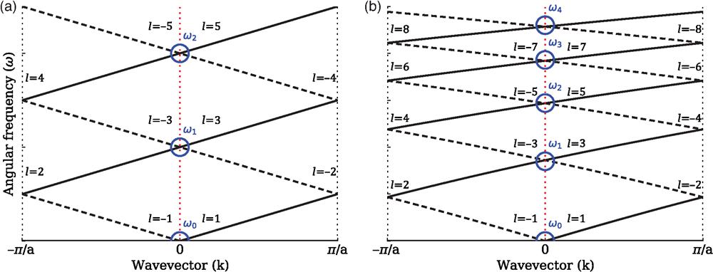
This dispersion relation corresponds to a straight band with band index and a slope , where is the (constant) refractive index. The bands with take the positive sign and correspond to light traveling in one direction. The bands with take the negative sign and correspond to light traveling in the other direction. We can include this information explicitly, making a positive integer:
These bands are graphically represented in Fig. 1(a) for the case of no material dispersion. Ring resonances appear when the bands intersect the line, which corresponds to field patterns with the right phase matching after one round trip. Explicitly, we see that
![]()
Figure 1.Photonic bands in an unperturbed ring resonator, plotted in a folded-zone diagram. A solid line corresponds to forward propagating bands, and a dashed line to backward-propagating ones. Each band is labeled with its corresponding band index. The resonances are marked when the bands cross the
This method is also applicable in case the medium has loss. In this particular case, we do it by replacing the refractive index by a phenomenological complex refractive index , where is the corresponding extinction coefficient (the extinction coefficient can include different loss mechanisms, such as material absorption, scattering, and diffraction losses). The resonance frequencies are now
Finally, the framework can be expanded to include dispersion by replacing the constant refractive index by a frequency-dependent one, ). This will cause the photonic bands to bend and then affect the resonance frequencies of the modes, as can be seen in the band diagram in Fig. 1(b).
3.2 Single-Frequency Perturbation
The unperturbed case works well, so we can move on to the simplest periodic perturbation over an average dielectric constant , one which has a single spatial frequency (where is a natural number). In this case, only three Fourier coefficients in Eq. (5) are non-zero, and we can write the coefficients as
For this perturbation, the central equation, Eq. (7), becomes
This is not a single equation, but rather an infinite family of coupled equations, one for each possible value of . Let us consider only two members of this family, the equations for :
The two equations above are linked to an infinite number of other equations due to the presence of the terms proportional to . For an unperturbed ring, as seen in Eq. (14), we can see that the frequency of the mode corresponding to is three times that of the modes for . If we consider a situation where only modes with frequencies near have a significant field amplitude (like for an excitation with a bandwidth much smaller than three times the frequency, which is a common occurrence at optical wavelengths), we can safely assume that the excitation of the modes will be negligible, and then we can set . Under this approximation, Eq. (20) becomes
We can find the new ’th photonic bands by solving for the roots of the above matrix’s characteristic polynomial, keeping only positive frequencies and finding that
Again, we find the modified resonances for the ’th modes evaluating the perturbed photonic bands at . The result is then
This result is exact, regardless of the amplitude of the perturbation. However, if the perturbation is small enough so that is satisfied, then we can expand the outer square root to the first order and obtain a simpler expression for the resonances,
For many relevant applications, a particularly important quantity is the gap between these two resonances, which is the perturbation-induced mode splitting. We can easily compute it from Eq. (25):
When the perturbation modifies the dielectric profile, but does not add any gain or loss to the system, then it will be modeled by a real function, and its Fourier coefficients will satisfy . Then, the magnitude of the induced mode splitting becomes
Furthermore, as long as resonant modes are excited with narrow-band light (with a bandwidth smaller than the FSR of the resonator, to avoid exciting more than one mode), we can extend the result from Eq. (26) to perturbations involving multiple Fourier coefficients, so that the splitting observed at a resonance with mode number is proportional to the product of the ’th and ’th Fourier coefficients of the perturbation.
For illustration purposes, let us consider an optical resonator constructed of a waveguide. As explored in Ref. 5, we can introduce a perturbation by modulating the waveguide width, leading to a position-dependent effective refractive index. Let us consider a harmonic modulation of the waveguide width, leading to an effective index
From the effective refractive index, we can define an effective dielectric constant ,
When the modulation is weak (), we can then approximate the inverse of the effective dielectric function as
Using the result from Eq. (25), then we can see that in a ring with such a perturbation, the mode with number (that is, with half the spatial frequency as the modulation), will then be split into two resonances with frequencies
If the modulation also introduces losses with the same spatial periodicity, the split-mode linewidths will also be affected. We can model this effect in a straightforward fashion by making both the mode frequency and the modulation amplitude complex. If and , then
In a typical microfabricated ring, in the optical telecommunications wavelength range, we will have , and (as long as no purposeful loss/gain modulation is introduced) we can expect that and will have a similar order of magnitude. In this case, Eq. (33) becomes somewhat simpler:
As previously mentioned, if we were to apply a modulation with more than one non-zero Fourier coefficient and use a narrowband light source so that only one resonant mode is excited, we can consider that each mode (with mode number ) will only be affected by the 2’th Fourier component modulation.
4 Experimental Results and Discussion
We designed modulated ring resonators based on waveguides on a integrated silicon nitride platform. The designed rings were fabricated by AEPONYX’s staff using their proprietary silicon nitride processes. The perturbations were implemented as a harmonic modulation of the waveguide width, as mentioned in the previous section, with the width varying as a function of the position along the ring as
We focused the study on a ring with a diameter, an average waveguide width of , and modulation amplitudes and (which will affect modes with and , respectively). A full view of the ring design, where the beating due to the presence of two Fourier coefficients can be observed, as well as a scanning electron microscope image of a fabricated ring can be seen in Fig. 2. The measurements were also made by AEPONYX staff. For each measurement, laser light was coupled into a waveguide in close proximity to a ring, and the transmission through this waveguide was measured as the wavelength of the laser was changed to obtain the spectral response. Grating couplers were used to interface the light source with the on-chip waveguide.
![]()
Figure 2.(a) Schematic of a waveguide-based ring having a width modulation with only two different non-zero Fourier coefficients. (b) Scanning electron microscope image of a fabricated silicon nitride ring and its coupling waveguide.
The experimentally measured spectra of a reference (unperturbed) ring and four rings with increasingly larger modulation amplitudes are shown in Fig. 3. The unperturbed ring has the characteristic ring resonator spectrum, with approximately equally spaced resonances, which have been assigned mode numbers from 61 to 65. As the values of the modulation amplitudes and are increased, reaching values of 150 nm each, we start seeing the expected splitting of the and modes while the other modes are not split. The ring with the 120-nm modulation amplitude does not show apparent mode splittings. This may be because the splitting is considerably smaller than the linewidth, and thus the two modes cannot be resolved from the data. The centers and linewidths of each resonant dip were extracted using a numerical peak-fitting tool,15 and factors were calculated from the fit parameters.
![]()
Figure 3.Experimental transmission spectrum of four different rings with different perturbation amplitudes. The bottom spectrum is that of an unperturbed ring, and the perturbation amplitudes increase going up (corresponding to 0-, 120-, 130-, 140-, and 150-nm width modulation amplitudes). The black lines correspond to the experimental data, and the thin red lines are the Lorentzian dips required to fit each corresponding mode. The traces are offset for visibility.
Tables 1 and 2 show the values of the mode splitting (when present) and the factors of the and modes. We can see that, for both modes, the higher perturbation amplitudes result in splittings, which are largest for the 150-nm modulation. Even though we did not purposefully introduce loss modulation, the split pairs also show asymmetry in their factors, with one mode having higher than the other. This tells us that the losses introduced by the waveguide width modulation possess a periodic component. For most modulation amplitudes, the high mode has less loss than the corresponding mode in the unperturbed ring, while the other has more loss. At the largest modulation amplitude, both factors become lower than the unperturbed one. This suggests that as the modulation increases the non-periodic losses also increase, reaching a point where they overwhelm the effect of the modulation on the linewidth. It is interesting to note that some of the modes in the modulated rings, which should have lower factors than those of the regular ring modes, actually show higher values (both modes with 120-nm modulation and the with 130-nm modulation). This happens because the non-modulated ring is more strongly coupled to the probing waveguide and thus subject to larger coupling losses. Rings with modulation amplitudes higher than 150 nm had so much loss that they did not show clear dips that could be reliably fit numerically.
| Modulation (nm) | Resonance splitting (nm) | ||||
| 0 | — | 349 | — | — | — |
| 120 | — | 472 | — | — | — |
| 130 | 1.9 | 335 | 1270 | ||
| 140 | 4.4 | 60 | 522 | ||
| 150 | 10.3 | 56 | 273 |
Table 1. Resonance splittings,
| Modulation (nm) | Resonance splitting (nm) | ||||
| 0 | — | 388 | — | — | — |
| 120 | — | 461 | — | — | — |
| 130 | 2.5 | 575 | 577 | ||
| 140 | 3.2 | 214 | 605 | ||
| 150 | 6.1 | 203 | 266 |
Table 2. Resonance splittings,
The tables also show values, calculated from the data using Eq. (34), for the real and imaginary parts of the perturbation coefficient . We can see that the value of increases as the modulation amplitude increases, qualitatively matching the expected trend from the model. The coefficient does not show a clear trend, which is consistent with losses introduced through unintentional fabrication defects.
5 Conclusions
We have introduced a formalism, inspired on those used to describe electrons in a solid crystal and extending the one presented in Ref. 5, to analyze the effect of perturbations on the resonant modes of an optical ring resonator. We discussed the case of a specific harmonic perturbation, where the formalism predicts that resonant modes with mode number will be split, with a splitting proportional to the ’th Fourier coefficient of the perturbation, and an asymmetry in the split-mode linewidths will be present. Experimental measurements of silicon nitride rings with width-modulated waveguides show good qualitative correspondence with the model predictions. This formalism provides interesting insights on the effect of general perturbations and could be used to analyze in further depth the effect of other experimentally important perturbations, such as nanoscale tips16 or nanoparticles.7
Kathleen McGarvey is a venture development specialist at TandemLaunch in Montreal, Quebec, Canada. She received her BSc from the University of Montana in 2010 and worked as a recruitment consultant in France for a few years. She earned her MSc degree in physics in 2015 and her PhD in physics in 2020, both from Concordia University, specializing in integrated photonics.
Pablo Bianucci is an associate professor in the Department of Physics at Concordia University in Montreal, Quebec, Canada. He received his Licenciado degree in physics from the Universidad de Buenos Aires in 2001 and his PhD in physics from the University of Texas at Austin in 2007. He worked as a postdoctoral fellow at the University of Alberta, McGill University, and École Polytechnique de Montréal. His current research interests are in the intersections of condensed matter and photonics, including topological photonics. He is a life member of SPIE.
References
[1] T. Ozawa et al. Topological photonics. Rev. Mod. Phys., 91, 015006(2019).
[4] H. Hodaei et al. Parity-time–symmetric microring lasers. Science, 346, 975-978(2014).
[13] K. Sakoda. Optical Properties of Photonic Crystals(2005).
[14] N. W. Ashcroft, N. D. Mermin. Solid State Physics(1976).

Set citation alerts for the article
Please enter your email address
© Copyright 2018-2021 | Chinese Laser Press. All Rights Reserved 沪ICP备15018463号-20