Experimental observations of boundary conditions of continuous-time quantum walks

Xiaochuan Han; Lantian Feng; Yuxuan Li; Lanxuan Zhang; Junfeng Song; Yongsheng Zhang

doi:10.3788/COL201917.052701

Abstract

The continuous-time quantum walk (CTQW) is the quantum analogue of the continuous-time classical walk and is widely used in universal quantum computations. Here, taking the advantages of the waveguide arrays, we implement large-scale CTQWs on chips. We couple the single-photon source into the middle port of the waveguide arrays and measure the emergent photon number distributions by utilizing the fiber coupling platform. Subsequently, we simulate the photon number distributions of the waveguide arrays by considering the boundary conditions. The boundary conditions are quite necessary in solving the problems of quantum mazes.

The continuous-time quantum walk (CTQW) was firstly investigated in 1998 by Farhi and Gutmann^[1,2]. Different from the discrete-time quantum walk (DTQW)^[3–5], neither the coin nor the coin operator is needed in CTQWs. The theoretical model of CTQWs originated from the continuous Markov process^[6–8], and thus, it is usually described by using graphs. The CTQWs are mostly used in universal quantum computations^[9–11], e.g., Childs et al. proposed an alternative quantum search algorithm based on CTQWs in 2003^[12]. Six years later, they also proposed a universal quantum computation method by using single-photon CTQWs in 2009^[10]. Solntsev et al. obtained different quantum correlations of one-dimensional (1D) CTQWs in nonlinear waveguide arrays in 2012^[13]. Caruso et al. used CTQWs to calculate the shortest route of escaping from a quantum maze in 2016^[14].

CTQWs are usually experimentally achieved in waveguide arrays. Obrien’s group firstly achieved two-photon CTQWs in 1D waveguide arrays in 2010^[15]. Three years later, they modified the scale of the structure to research the coherent time evolution and boundary conditions of two-photon CTQWs in the 808 nm band. In 2014, they experimentally achieved two-dimensional (2D) CTQWs in swiss-cross waveguides^[16]. In 2018, Jin’s group experimentally observed single-photon CTQWs in a $49 \times 49$ port photonic chip^[17]. Up to now, the researches of CTQWs are extended to multiple dimensions and are large-scale.

When considering CTQWs in finite-sized waveguide arrays, the boundary conditions cannot be neglected. Although some previous researches have reported the boundary conditions in some degree, they have not given a quantitative analysis. In this Letter, we experimentally measure single-photon CTQWs in two kinds of silicon waveguide arrays, which are different in the coupling distance by the fiber coupling platform. Through calculating the coupling length of the nearest waveguides, we can simulate the nearest coupling constant. Using these results, we can simulate the photon number distributions. We compare them with the experimental ones and quantitatively analyze the boundary conditions. In solving the problem, such as quantum mazes or complicated quantum gates, as long as the photons propagate to the boundary, the boundary condition is quite necessary to be considered.

Sign up for Chinese Optics Letters TOC. Get the latest issue of Chinese Optics Letters delivered right to you！Sign up now

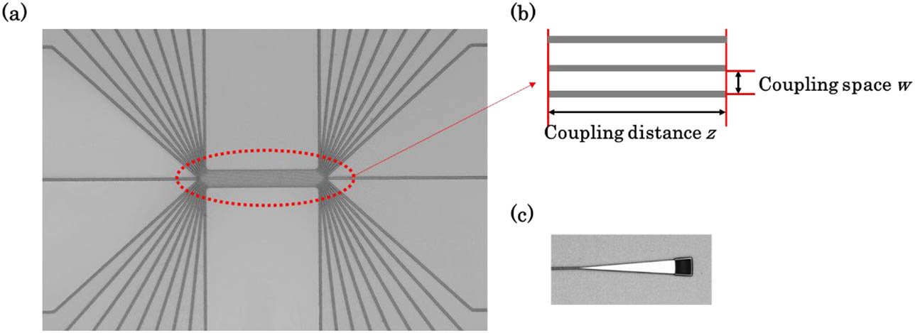
The silicon optical chip has the advantages of small size, high coupling efficiency, low loss, and high stability^[18–20]. Because of the specific nature of silicon, the chip is widely used in the communication band. The CTQWs are implemented by using multiple waveguides coupling on chips, which are shown in the red circle of Fig. 1(a). The width of the waveguide is 0.5 μm. The other two parameters of the waveguide that can be modified in this experiment are the coupling distance $z$ and the coupling space $w$ , which are shown in Fig. 1(b). The incident and emergent light is coupled by using an optical grating, which is shown in Fig. 1(c).

Figure 1.(a) Microphotograph of nineteen waveguides that are coupled together to be used for CTQWs. (b) The detailed description of the coupling distance $z$ and the coupling space $w$ . (c) Microphotograph of the optical grating that is used for light coupling.

Due to the fact that the silicon waveguides have a height of only 220 nm, TE CTQWs are implemented in this experiment. The output coincidence counts are measured by fiber coupling platform^[21], which is shown in Fig. 2. The wavelength of the incident photon pairs we use is 1550 nm, which are generated by the 775 nm continuous laser via a periodically poled potassium titanyl phosphate (PPKTP) crystal. Then, the photon pairs are separated by the polarization beam splitter (PBS). One of the photon pairs is coupled into the chip via the optical grating on the chip for CTQWs and finally detected by the superconducting nanowire single-photon detector 1 (SNSPD1), while the other one is detected without CTQWs by SNSPD2. The arrival time of the photons is modified for the coincidence counting. The coincidence rates are about 150,000 per second, and the counting time of the detection is 3 s. The experimental probability distributions are displayed in the red bars of Figs. 3(b), 4(b)–4(e).

Figure 2.Experimental set-up of the fiber coupling platform. The continuous-wave pump laser at 775 nm from a Ti:sapphire laser (Coherent MBR 110) is transferred by a single-mode fiber (SMF). A pair of quarter wave plate (QWP) and half wave plate (HWP) is used for phase modification. The PBS is used to separate the photon of different polarizations. Lenses (L) are used to focus the photon into the type II PPKTP for generating 1550 nm photon pairs. The dichroic mirror (DM) and the long pass filter (LPF) are used to purify the pump beams. After walking through the waveguide arrays on the chip, the polarization controller (PC) is used to modify the polarization. All of the photons are detected by SNSPDs and are finally coincidence counted.

Figure 3.(a) Simulated probability distribution of the single-photon source injected into the central waveguide array as a function of the coupling distance. (b) The calculated (blue) and experimental (red) probability distribution of CTQWs with $w = 0.3 μm$ and $z = 100 μm$ .

Figure 4.(a) Image computation method of CTQWs in a limited region. The calculated (blue) and experimental (red) probability distribution of (b) third port incident, (c) fifth port incident, (d) seventh port incident, and (e) tenth port incident CTQWs with $w = 0.3 μm$ , $z = 800 μm$ .

The results of CTQWs are simulated by using the Bessel function^[22], and we only consider the nearest coupling here. The output creation operator can be written as $a_{m}^{+} (z) = e^{i β z} i^{m - j} J_{m - j} (2 c z) a_{j}^{+} (0),$ (1)where $a_{j}^{+} (0)$ and $a_{m}^{+} (z)$ are the creation operators of the start and the end, $c$ is the coupling constant of the nearest neighbor, $z$ is the coupling distance, $β$ is the propagation constant, $j$ is the number of the incident waveguide, and $m$ is the number of the emergent waveguide. Using Eq. (1), we can obtain the output photon number distribution of the waveguide structure in Fig. 3(a). The parameters of the waveguide structure we use are $w = 0.3 μm$ and $z = 100 μm$ , and the calculated photon number distributions are shown in the blue bars of Fig. 3(b). We obtain the coupling length and the coupling constant by resorting to the beam propagation method (BPM). When $w = 0.3 μm$ , the coupling length is 106 μm, and the coupling constant is $c = 0.0148 {μm}^{- 1}$ . As the single-photon source is coupled into the middle port and the coupling distances are short, the photon will not walk to the boundary of the structure. The photon number distribution is extending symmetrically as the coupling distance $z$ increases.

If we modify the parameter of the structure, in other words, when considering a limit region, the walker will be reflected at the boundary. Thus, when we calculated this structure, we need to use the image method^[23]. As we show in Fig. 4(a), the images are placed symmetrically about the boundaries with the walker. We suppose the images are also walkers and walk together with the real walker. However, this walk is not real, so we need to add a negative sign, and the output creation operator can be written as $a_{m}^{+} (z) = e^{i β z} [i^{m - j} J_{m - j} (2 c z) - i^{m + j} J_{m + j} (2 c z) - i^{m + j - 40} J_{m + j - 40} (2 c z)] a_{j}^{+} (0),$ (2)where the first item in the bracket is the real walker, and the second and the third are the image walkers of both sides. By using Eq. (2), we can calculate probability distributions of CTQWs with boundary conditions. Here, the coupling space of the structure we use is 0.3 μm, and the coupling distance is 800 μm so that we can ensure that the photon can walk over the boundary. The CTQWs are obtained by coupling the single-photon source into the 3rd, 5th, 7th, and 10th port of the waveguide. Thus, the calculated probability distributions are shown in the blue bars in Figs. 4(b)–4(e). We use the fidelities^[24] to evaluate the results, which can be written as $F = \sum_{i = 1}^{n} \sqrt{P_{1 i} P_{2 i}},$ (3)where $F$ is the fidelity, $n$ is the number of ports, $P_{1 i}$ and $P_{2 i}$ are the calculated and experimental probability distributions of the $i$ th port. $F_{1} = 0.8609$ (tenth port incident, $w = 0.3 μm$ , $z = 100 μm$ ), $F_{2} = 0.8498$ (third port incident, $w = 0.3 μm$ , $z = 800 μm$ ), $F_{3} = 0.8237$ (fifth port incident, $w = 0.3 μm$ , $z = 800 μm$ ), $F_{4} = 0.8969$ (seventh port incident, $w = 0.3 μm$ , $z = 800 μm$ ), and $F_{5} = 0.8722$ (tenth port incident, $w = 0.3 μm$ , $z = 800 μm$ ). Although there is a length difference between the output channels, the transmission loss of the waveguide (1.5 dB/cm) that can be almost neglected is very low, considering the length of our system. However, the coupling loss is relatively large, and the coupling efficiency of each port is different, which will cause errors in some degree. In addition, other errors are caused by the small difference in the spacing and length of the waveguides.

The probability distributions depend on the two parameters, $c$ and $z$ . $c$ determines the diffusion velocity per unit distance, and $z$ is the distance. Thus, $c \cdot z$ determines the total probability distributions.

In this Letter, we summarize the image method in solving the boundary conditions of photon transmission in finite-sized waveguide arrays and apply it by using CTQWs in two waveguide structures with different parameters. We use one of them to observe CTQWs with boundary conditions and the other one to observe CTQWs without boundary conditions. The experiment of these CTQWs is done by injecting the 1550 nm single-photon source into the waveguides and measuring it with the fiber coupling platform. The simulated results of the CTQW without boundary conditions are done by using Bessel functions, while the results of the CTQW with boundary conditions are simulated by using the image method in order to consider the boundary conditions. The experimental results have high fidelities with the simulated ones. Therefore, the boundary conditions are quite necessary in solving the problem of the quantum maze or other large-scale quantum computations, and using the image method is an effective way to obtain the simulated results. For further researches, we will pay more attention to the boundary of more complicated CTQWs on chips.

References

[1] E. Farhi, S. Gutmann. Phys. Rev.A, 58, 915(1998).

[2] J. Kempe. Contemp. Phys., 50, 339(2009).

[3] G. Mastio, P. Milman. Quantum Information and Measurement (QIM) 2017, QT6A.31(2017).

[4] A. M. Childs. Commun. Math. Phys., 294, 581(2010).

[5] N. Konno. Quantum Inf. Process., 9, 405(2010).

[6] A. Romanelli. Phys. Rev. A, 81, 44(2010).

[7] A. Romanelli(2010).

[8] A. Romanelli, A. C. S. Schifino, R. Siri, G. Abal, A. Auyuanet, R. Donangelo. Phys. A Stat. Mech. Appl., 338, 395(2003).

[9] M. Mottonen, J. J. Vartiainen, V. Bergholm, M. M. Salomaa(2004).

[10] A. M. Childs. Phys. Rev. Lett., 102, 180501(2009).

[11] C. Zhou, C. Zhang, H. Liu, K. Liu, H. Sun, J. Gao. Chin. Opt. Lett., 15, 092703(2017).

[12] A. M. Childs, J. Goldstone. Phys. Rev. A, 70, 690(2003).

[13] A. S. Solntsev, A. A. Sukhorukov, D. N. Neshev, Y. S. Kivshar. Phys. Rev. Lett., 108, 023601(2012).

[14] F. Caruso, A. Crespi, A. G. Ciriolo, F. Sciarrino, R. Osellame. Nat. Commun., 7, 11682(2016).

[15] A. Peruzzo, M. Lobino, J. C. F. Matthews, N. Matsuda, A. Politi, K. Poulios, X.-Q. Zhou, Y. Lahini, N. Ismail, K. Wörhoff, Y. Bromberg, Y. Silberberg, M. G. Thompson, J. L. O’Brien. Science, 329, 1500(2010).

[16] K. Poulios, R. Keil, D. Fry, J. D. Meinecke, J. C. Matthews, A. Politi, M. Lobino, M. Heinrich, S. Nolte, A. Szameit. Phys. Rev. Lett., 112, 143604(2014).

[17] H. Tang, X. F. Lin, Z. Feng, J. Y. Chen, J. Gao, K. Sun, C. Y. Wang, P. C. Lai, X. Y. Xu, Y. Wang, L.-F. Qiao, A.-L. Yang, X.-M. Jin. Sci. Adv., 4, eaat3174(2018).

[18] Y. Huang, C. Guo, R. Bao, X. Wang. Chin. Opt. Lett., 11, 052201(2013).

[19] J. Yang, P. Bhattacharya, Z. Mi, G. Qin, Z. Ma. Chin. Opt. Lett., 6, 727(2008).

[20] V. R. Almeida, C. A. Barrios, R. R. Panepucci, M. Lipson. Nature, 431, 1081(2004).

[21] L. T. Feng, M. Zhang, Z. Y. Zhou, M. Li, X. Xiong, L. Yu, B. S. Shi, G. P. Guo, D. X. Dai, X. F. Ren. Nat. Commun., 7, 11985(2016).

[22] D. Ben-Avraham, E. M. Bollt, C. Tamon. One-Dimensional Continuous-Time Quantum Walks, 295(2004).

[23] K. G. Makris, D. N. Christodoulides. Phys. Rev. E Stat. Nonlinear Soft Matter Phys., 73, 036616(2006).

[24] X. C. Han, D. W. Zhuang, Y. X. Li, J. F. Song, Y. S. Zhang. Chin. Phys. B, 27, 74208(2018).