• Acta Physica Sinica
  • Vol. 69, Issue 7, 077102-1 (2020)
Peng Ye*
Author Affiliations
  • School of Physics, Sun Yat-sen University, Guangzhou 510275, China
  • show less
    DOI: 10.7498/aps.69.20200197 Cite this Article
    Peng Ye. Gauge theory of strongly-correlated symmetric topological Phases[J]. Acta Physica Sinica, 2020, 69(7): 077102-1 Copy Citation Text show less
    Monte Carlo verification of vanishing topological entanglement entropy of the SPT wave function obtained from the projective construction
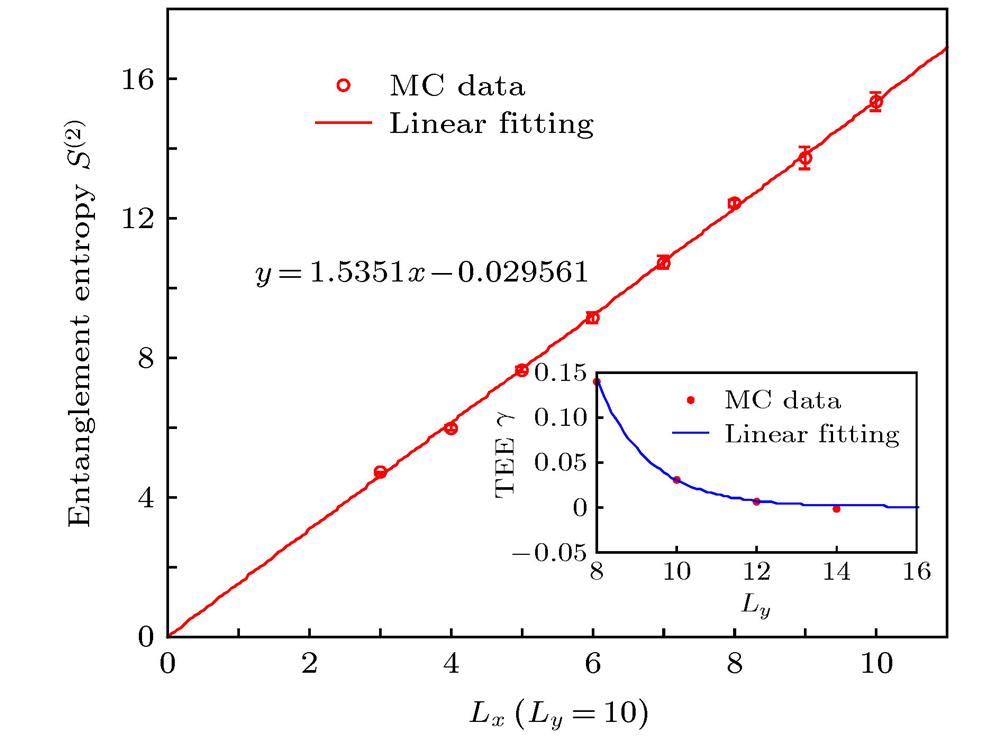
    Fig. 1. Monte Carlo verification of vanishing topological entanglement entropy of the SPT wave function obtained from the projective construction
    Parton decomposition of electron operators
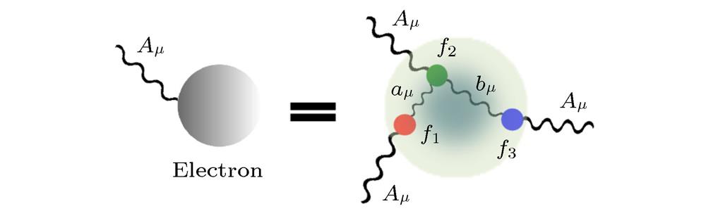
    Fig. 2. Parton decomposition of electron operators
    Diagrammatic illustration of fusion rules among twist defects and topological excitations. (a) Fusions between an anyon (quasiparticle) and a point-defect in a two-dimensional iTO. (b) Fusions between a particle excitation and a line defect in a three-dimensional iTO; (c) Fusions between a loop excitation and a line defect in a three-dimensional iTO.[85]
    Fig. 3. Diagrammatic illustration of fusion rules among twist defects and topological excitations. (a) Fusions between an anyon (quasiparticle) and a point-defect in a two-dimensional iTO. (b) Fusions between a particle excitation and a line defect in a three-dimensional iTO; (c) Fusions between a loop excitation and a line defect in a three-dimensional iTO.[85]
    Illustration of gauge-invariant Wilson operators in Eq. (26)
    Fig. 4. Illustration of gauge-invariant Wilson operators in Eq. (26)
    Illustration of point-like excitations and loop excitations in three-dimensional iTO
    Fig. 5. Illustration of point-like excitations and loop excitations in three-dimensional iTO
    (a) Particle-loop braiding: a particle travels around a loop such that the braiding trajectory and form a Hopf link. (b) Borromean-Rings braiding: a particle moves around two unlinked loops such that , and the trajectory form the Borromean rings (or generally the Brunnian link)
    Fig. 6. (a) Particle-loop braiding: a particle travels around a loop such that the braiding trajectory and form a Hopf link. (b) Borromean-Rings braiding: a particle moves around two unlinked loops such that , and the trajectory form the Borromean rings (or generally the Brunnian link)
    Illustration of SEG
    Fig. 7. Illustration of SEG
    (a). Topological response for Eq. (42). The intersection of and symmetry domain walls and carries the angular momentum . and are the gauge connections normal to the domain walls. (b). Topological response of Eq. (44). The intersection of disclination line and symmetry domain walls carries the charge . and are the gauge connections normal to the disclination line and domain wall, respectively
    Fig. 8. (a). Topological response for Eq. (42). The intersection of and symmetry domain walls and carries the angular momentum . and are the gauge connections normal to the domain walls. (b). Topological response of Eq. (44). The intersection of disclination line and symmetry domain walls carries the charge . and are the gauge connections normal to the disclination line and domain wall, respectively
    Illustration of two examples of SPT topological response phenomena in three dimensions
    Fig. 9. Illustration of two examples of SPT topological response phenomena in three dimensions
    拟设完全被 $f_1$填充的陈-能带 完全被 $f_2$填充的陈-能带 自旋矢量 $q^T_s$电荷矢量 $q^T_c$
    $A1$$\uparrow+, \downarrow+, \uparrow-, \downarrow-$$(2, 2)$$\uparrow+, \downarrow+, \uparrow-, \downarrow-$$(2, 2)$$\left(\dfrac{1}{2}~~-\dfrac{1}{2}~~\dfrac{1}{2}~~-\dfrac{1}{2}~~\dfrac{1}{2}~~-\dfrac{1}{2}~~\dfrac{1}{2}~~-\dfrac{1}{2}\right)$$(1~~1~~1~~1~~1~~1~~1~~1)$
    $A2$$\uparrow+, \downarrow-$$(1, 1)$$\uparrow+, \downarrow-$$(1, 1)$$\left( {1}/{2}~~- {1}/{2}~~ {1}/{2}~~ -{1}/{2}\right)$$(1~~1~~1~~1)$
    $A3$$\uparrow+, \downarrow-$$(1, 1)$$\downarrow+, \uparrow-$$(1, 1)$$\left(1/{2}~~- {1}/{2}~~- {1}/{2}~~ {1}/{2}\right)$$(1~~1~~1~~1)$
    $A4$$\uparrow+, \downarrow-$$(1, 1)$$\left( {1}/{2}~~- {1}/{2}\right)$$(1~~1)$
    Table 1. Parton ansatzes in the two-dimensional projective construction. stand for four different ansatzes respectively. Each fully occupied band is labeled by a pair of arrow and plus/minus sign. The arrow represents the spin eigenvalue of , and represents Chern number . In A1, there are 8 fully occupied Chern bands; There are 4 fully occupied Chern bands in each of A2 and A3. In A4, flavor index is not involved, so only one flavor, say, is taken into account. And there are two filled Chern bands. A pair of integers denote the filling number of either and in each unit cell: (fermion number with up spin, fermion number with down spin).
    U任意一个格点上的物理希尔伯特空间基矢 $ [f_1]n_{i, 1 \uparrow}, n_{i, 1 \downarrow}, n_{i, 2 \uparrow}, n_{i, 2 \downarrow}[f_2] $费米子填充总数要求
    $U_1$$(0, 0, 0, 0)$, $(0, 1, 0, 1)$, $(0, 1, 1, 0)$, $(1, 0, 0, 1)$, $(1, 0, 1, 0)$, $(1, 1, 1, 1)\, $$N^{f1}=N^{f2} $
    $U_2$$(0, 0, 0, 0)$, $(0, 1, 1, 0)$, $(1, 0, 0, 1)$, $(1, 1, 1, 1)\, $$N^{f1}_{\uparrow} = N^{f2}_{\downarrow}, $$N^{f1}_{\downarrow}=N^{f2}_{\uparrow}$
    $U_3$$(0, 0, 0, 0)$, $(0, 1, 0, 1)$, $(1, 0, 1, 0)$, $(1, 1, 1, 1)\, $$N^{f1}_{ \uparrow}=N^{f2}_{ \uparrow}, $$N^{f1}_{ \downarrow}=N^{f2}_{\downarrow}$
    $U_4$$(0, 0, 1, 1)$, $(0, 1, 0, 1)$, $(1, 0, 1, 0)$, $(1, 1, 0, 0)$$N^{f1}_{\uparrow}+N^{f2}_{\downarrow}=N_{\rm latt}$, $N^{f2}_{\uparrow}+ N^{f1}_{\downarrow}=N_{\rm att}$
    $U_5$$(1, 0, 0, 0)$, $(0, 1, 0, 0)$, $(0, 0, 1, 0)$, $(0, 0, 0, 1)$$ N^{f1} + N^{f2}=N_{\rm latt}$
    $U_6$$(1, 0)$, $(0, 1)$$ N^{f1} =N_{\rm latt}$
    $U_7$$(0, 0)$, $(1, 1)$$N^{f1}_{\uparrow} = N^{f1}_{\downarrow }$
    Table 2.

    At large U limit, the physical Hilbert space is formed by those occupancy bases without energy cost. We should restrict the total particle number of each flavor properly such that Hilbert space of every site is always in the physical Hilbert space

    在大U极限下, 实空间每个格点上的不消耗U能量的占据状态形成了物理希尔伯特空间. 我们需要对费米子的总的填充数做限制. 限制之后, 所有格点都能够同时处于物理希尔伯特空间.

    对称群G拓扑规范场论与分类
    $\mathbb{Z}_{N_1}\times\mathbb{Z}_{N_2}$$\dfrac{1}{2{\text{π}}}\displaystyle\int \sum^2_Ib^I\wedge \, {\rm d}a^I+ p_1\displaystyle\int a^1\wedge a^2\wedge \, {\rm d}a^2~~(\mathbb{Z}_{N_{12}} )$ ; $\dfrac{1}{2{\text{π}}}\displaystyle\int \sum^2_Ib^I\wedge \, {\rm d}a^I+ p_2\displaystyle\int a^2\wedge a^1\wedge \, {\rm d}a^1 ~(\mathbb{Z}_{N_{12}}) $
    $\mathbb{Z}_{N_1}\times\mathbb{Z}_{N_2}\times\mathbb{Z}_{N_3} $$\dfrac{1}{2{\text{π}}}\displaystyle\int \sum^3_Ib^I\wedge \, {\rm d}a^I+ p_1 \displaystyle\int a^1\wedge a^2\wedge \, {\rm d}a^3~~(\mathbb{Z}_{N_{123}})$ ; $\dfrac{1}{2{\text{π}}}\displaystyle\int \sum^3_Ib^I\wedge \, {\rm d}a^I+ p_2 \displaystyle\int a^2\wedge a^3\wedge \, {\rm d}a^1~~(\mathbb{Z}_{N_{123}}) $
    $\prod^4_I\mathbb{Z}_{N_I} $$\dfrac{1}{2{\text{π}}}\displaystyle\int \sum^4_Ib^I\wedge \, {\rm d}a^I+p \displaystyle\int a^1\wedge a^2\wedge a^3\wedge a^4~~ ( \mathbb{Z}_{N_{1234}} )$
    $\mathbb{Z}_{N_1}\times\mathbb{Z}_{N_2}\times {U}(1)$$\dfrac{1}{2{\text{π}}}\displaystyle\int \sum^3_Ib^I\wedge \, {\rm d}a^I+p\displaystyle\int a^1\wedge a^2\wedge \, {\rm d}a^3~~ (\mathbb{Z}_{N_{12}})$
    Table 3. A brief summary of irreducible 3D SPT phases with unitary Abelian symmetry. and are 1-form and 2-form gauge fields, respectively. “( ) ”denote the corresponding classifications, where are greatest common divisors of . SPT phases with either or or are trivial and not included below. By “irreducible”, we means that all subgroups of symmetry group play nontrivial roles in protecting the nontrivial SPT phases. All other SPT's with unitary Abelian group symmetries can be obtained directly by using this table[129].
    规范群 $G_g$twisted拓扑项对称群 $G_s$SET分类
    ${\mathbb{Z}}_2$${\mathbb{Z}}_{2 n + 1}$${{\mathbb{Z}}_1}$
    ${\mathbb{Z}}_2$${\mathbb{Z}}_{2 n}$$ {({\mathbb{Z}}_2)^2}\oplus {\mathbb{Z}}_1$
    ${\mathbb{Z}}_3$${\mathbb{Z}}_{3 n}$$({\mathbb{Z}}_3)^2\oplus {\mathbb{Z}}_1 \oplus {\mathbb{Z}}_1$
    ${\mathbb{Z}}_3$${\mathbb{Z}}_{3 n + 1}$${\mathbb{Z}}_1$
    ${\mathbb{Z}}_4$${\mathbb{Z}}_{2 n + 1}$${\mathbb{Z}}_1$
    ${\mathbb{Z}}_4$${\mathbb{Z}}_{4 n+2}$$ ({\mathbb{Z}}_2)^2\oplus {\mathbb{Z}}_1$
    ${\mathbb{Z}}_4$${\mathbb{Z}}_{4 n}$$ ({\mathbb{Z}}_4)^2\oplus ({\mathbb{Z}}_2)^2\oplus {\mathbb{Z}}_1 \oplus {\mathbb{Z}}_1 $
    ${\mathbb{Z}}_2\times {\mathbb{Z}}_2$(0, 0)${\mathbb{Z}}_{2 n}$$({\mathbb{Z}}_2)^6\oplus ({\mathbb{Z}}_2)^2 \oplus ({\mathbb{Z}}_2)^2 \oplus ({\mathbb{Z}}_2)^2$
    ${\mathbb{Z}}_2\times {\mathbb{Z}}_2$(0, 0)${\mathbb{Z}}_{2 n + 1}$${\mathbb{Z}}_1$
    ${\mathbb{Z}}_2\times {\mathbb{Z}}_2$(2, 0)${\mathbb{Z}}_{2 n}$$({\mathbb{Z}}_2)^6$
    ${\mathbb{Z}}_2\times {\mathbb{Z}}_2$(2, 0)${\mathbb{Z}}_{2 n + 1}$${\mathbb{Z}}_1$
    ${\mathbb{Z}}_2\times {\mathbb{Z}}_2$(2, 2)${\mathbb{Z}}_{2 n + 1}$${\mathbb{Z}}_1$
    ${\mathbb{Z}}_2\times {\mathbb{Z}}_4$(0, 0)${\mathbb{Z}}_{2 n + 1}$${\mathbb{Z}}_1$
    ${\mathbb{Z}}_2\times {\mathbb{Z}}_4$(4, 0)${\mathbb{Z}}_{2 n + 1}$${\mathbb{Z}}_1$
    ${\mathbb{Z}}_2\times {\mathbb{Z}}_4$(4, 4)${\mathbb{Z}}_{2 n + 1}$${\mathbb{Z}}_1$
    ${\mathbb{Z}}_2\times {\mathbb{Z}}_4$(0, 0)${\mathbb{Z}}_{4 n}$$({\mathbb{Z}}_2)^4\times ({\mathbb{Z}}_4)^2\oplus 2({\mathbb{Z}}_4)^2\oplus4({\mathbb{Z}}_2)^2 \oplus ({\mathbb{Z}}_2)^6$
    ${\mathbb{Z}}_2\times {\mathbb{Z}}_4$(4, 0)${\mathbb{Z}}_{4 n}$$({\mathbb{Z}}_2)^4\times ({\mathbb{Z}}_4)^2$
    ${\mathbb{Z}}_2\times {\mathbb{Z}}_4$(4, 4)${\mathbb{Z}}_{4 n}$$({\mathbb{Z}}_2)^4\times ({\mathbb{Z}}_4)^2$
    ${\mathbb{Z}}_2$${\mathbb{Z}}_{2 m + 1} \times {\mathbb{Z}}_{2 n + 1}$$({\mathbb{Z}}_{2\gcd(2 m + 1, 2 n + 1)})^2$
    ${\mathbb{Z}}_2$${\mathbb{Z}}_{2 m + 1} \times {\mathbb{Z}}_{2 n}$$({\mathbb{Z}}_{\gcd(2 m + 1, 2 n)})^2 \oplus ({\mathbb{Z}}_{2\gcd(2 m + 1, 2 n)})^2 $
    ${\mathbb{Z}}_2$${\mathbb{Z}}_{2 m} \times {\mathbb{Z}}_{2 n}$$({\mathbb{Z}}_2)^6\times({\mathbb{Z}}_{2\gcd(m, n)})^2\oplus ({\mathbb{Z}}_{2\gcd(2 m, n)})^2 \oplus ({\mathbb{Z}}_{2\gcd(m, 2 n)})^2 \oplus ({\mathbb{Z}}_{2\gcd(m, n)})^2$
    ${\mathbb{Z}}_4$${\mathbb{Z}}_{2 n + 1} \times {\mathbb{Z}}_{2 n + 1}$$16({\mathbb{Z}}_{2 n + 1})^2$
    ${\mathbb{Z}}_4$${\mathbb{Z}}_{2(2 n + 1)} \times {\mathbb{Z}}_{2(2 n + 1)}$$4({\mathbb{Z}}_2)^6 \times ({\mathbb{Z}}_{2(2 n + 1)})^2\oplus 12({\mathbb{Z}}_{2(2 n + 1)})^2$
    ${\mathbb{Z}}_4$${\mathbb{Z}}_{4 n} \times {\mathbb{Z}}_{4 n}$$({\mathbb{Z}}_4)^6 \times ({\mathbb{Z}}_{4 n})^2\oplus 12({\mathbb{Z}}_{4 n})^2 \oplus 3[ ({\mathbb{Z}}_{4 n})^2\times ({\mathbb{Z}}_2)^6]$
    ${\mathbb{Z}}_2\times {\mathbb{Z}}_2$(0, 0)${\mathbb{Z}}_{2}\times {\mathbb{Z}}_2$$({\mathbb{Z}}_2)^{18}\oplus 6({\mathbb{Z}}_2)^8 \oplus 3({\mathbb{Z}}_2)^6 \oplus 6({\mathbb{Z}}_2)^4$
    ${\mathbb{Z}}_2\times {\mathbb{Z}}_2$(2, 0)${\mathbb{Z}}_{2}\times {\mathbb{Z}}_2$$({\mathbb{Z}}_2)^{18}$
    ${\mathbb{Z}}_2\times {\mathbb{Z}}_2$(2, 2)${\mathbb{Z}}_{2}\times {\mathbb{Z}}_2$$({\mathbb{Z}}_2)^{18}$
    Table 4.

    Classification of SET examples.

    部分三维SET的分类, 摘自[50].

    投影对称群(PSG)规范群 $G_g$对称群 $G_s$三维体内( $\varSigma^3$) 的规范理论 表面( $\partial\varSigma^3$)的反常 玻色理论 二维平面( $\varSigma^2$)的正常Chern-Simons理论的 $K_G$-矩阵
    ${\mathbb{Z}}_N \rtimes{\mathbb{Z}}^T_2$${\mathbb{Z}}_N$${\mathbb{Z}}^T_2$$\dfrac{N}{4{\text{π}}} \epsilon^{\mu\nu\lambda\rho} B^c_{\mu\nu}\partial_\lambda A_\rho^c+$$\dfrac{\theta_c}{8{\text{π}}^2} \epsilon^{\mu\nu\lambda\rho}\partial_\mu A^c_\nu \partial_\lambda A^c_\rho$${\mathbb{Z}}^T_2$破缺的 $\partial\varSigma^3$: $\dfrac{N}{2{\text{π}}}\partial_0 \phi^c \epsilon^{ij}\partial_i \lambda^c_j$${\mathbb{Z}}^T_2$破缺的 $\varSigma^2$: $\left(\begin{array}{*{20}{c}} {2 p}&N\\ N&0 \end{array}\right)$
    ${\mathbb{Z}}_N\!\times\!{\mathbb{Z}}^T_2$${\mathbb{Z}}_N$${\mathbb{Z}}^T_2$$\dfrac{N}{4{\text{π}}} \epsilon^{\mu\nu\lambda\rho} B^s_{\mu\nu}\partial_\lambda A_\rho^s+$$\dfrac{\theta_s}{8{\text{π}}^2} \epsilon^{\mu\nu\lambda\rho}\partial_\mu A^s_\nu \partial_\lambda A^s_\rho$${\mathbb{Z}}^T_2$破缺的 $\partial\varSigma^3$: $\dfrac{N}{2{\text{π}}}\partial_0 \phi^s \epsilon^{ij}\partial_i \lambda^s_j$${\mathbb{Z}}^T_2$破缺的 $\varSigma^2$: $ \left({\begin{array}{*{20}{c}} 2 p &N \\ N & 0 \end{array}} \right)$
    ${\mathbb{Z}}_N \!\times\! [U(1)_{S^z}\rtimes{\mathbb{Z}}_2]$${\mathbb{Z}}_N\!\times\! U(1)_{S^z}$${\mathbb{Z}}_2$$\dfrac{N}{4{\text{π}}} \epsilon^{\mu\nu\lambda\rho} B^c_{\mu\nu}\partial_\lambda A_\rho^c +$$\dfrac{\theta_0}{4{\text{π}}^2} \epsilon^{\mu\nu\lambda\rho}\partial_\mu A^s_\nu \partial_\lambda A^c_\rho$${\mathbb{Z}}_2$破缺的 $\partial\varSigma^3$: $\dfrac{N}{2{\text{π}}}\partial_0 \phi^c \epsilon^{ij}\partial_i \lambda^c_j$${\mathbb{Z}}_2$破缺的 $\varSigma^2$: $ \left({\begin{array}{*{20}{c}} 2 p_1 &N & p_{12}& 0\\ N & 0 &0 & 0\\ p_{12} & 0 &2 p_2 & 0\\ 0 & 0 &0 & 0 \end{array}} \right)$
    $U(1)_C \!\times\! [{\mathbb{Z}}_N \rtimes{\mathbb{Z}}_2]$$U(1)_C\!\times\!{\mathbb{Z}}_N$${\mathbb{Z}}_2$$\dfrac{N}{4{\text{π}}} \epsilon^{\mu\nu\lambda\rho} B^s_{\mu\nu}\partial_\lambda A_\rho^s+$$\dfrac{\theta_0}{4{\text{π}}^2} \epsilon^{\mu\nu\lambda\rho}\partial_\mu A^s_\nu \partial_\lambda A^c_\rho$${\mathbb{Z}}_2$破缺的 $\partial\varSigma^3$: $\dfrac{N}{2{\text{π}}}\partial_0 \phi^s \epsilon^{ij}\partial_i \lambda^s_j$${\mathbb{Z}}_2$破缺的 $\varSigma^2$: $ \left({\begin{array}{*{20}{c}} 2 p_1 &0 & p_{12}& 0\\ 0 & 0 &0 & 0\\ p_{12} & 0 &2 p_2 & N\\ 0 & 0 &N & 0 \end{array}} \right)$
    ${\mathbb{Z}}_{N_1} \!\times\! [{\mathbb{Z}}_{N_2}\rtimes{\mathbb{Z}}_2]$${\mathbb{Z}}_{N_1}\!\times\! {\mathbb{Z}}_{N_2}$${\mathbb{Z}}_2$$\dfrac{N_1}{4{\text{π}}} \epsilon^{\mu\nu\lambda\rho} B^c_{\mu\nu}\partial_\lambda A_\rho^c+$$\dfrac{N_2}{4{\text{π}}} \epsilon^{\mu\nu\lambda\rho} B^s_{\mu\nu}\partial_\lambda A_\rho^s+$$\dfrac{\theta_0}{4{\text{π}}^2} \epsilon^{\mu\nu\lambda\rho}\partial_\mu A^s_\nu \partial_\lambda A^c_\rho$${\mathbb{Z}}_2$破缺的 $\partial\varSigma^3$: $\dfrac{N_1}{2{\text{π}}}\partial_0 \phi^c \epsilon^{ij}\partial_i \lambda^c_j+$$\dfrac{N_2}{2{\text{π}}}\partial_0 \phi^s \epsilon^{ij}\partial_i \lambda^s_j$${\mathbb{Z}}_2$破缺的 $\varSigma^2$: $\begin{aligned} & {}\\ & \left({\begin{array}{*{20}{c}} 2 p_1 &N_1 & p_{12}& 0\\ N_1 & 0 &0 & 0\\ p_{12} & 0 &2 p_2 & N_2\\ 0 & 0 &N_2 & 0 \end{array}} \right)\end{aligned}$
    Table 5.

    Bulk and boundary theories of SET with anti-unitary symmetry (e.g., time-reversal symmetry).

    部分含有反幺正对称群(时间反演)的SET的体内理论与边界理论, 摘自[51].

    轴子角对称群三维体内( $\varSigma^3$)的响应 二维表面( $\partial\varSigma^3$)的反常响应 二维平面( $\varSigma^2$)的响应
    $ \theta_c=2{\text{π}}+4{\text{π}} k$ (带电玻色系统) $U(1)_C\rtimes{\mathbb{Z}}^{\rm T}_2$电荷-威腾效应: $N^c=n^c+N^c_m$量子电荷霍尔效应 ( ${\mathbb{Z}}^{\rm T}_2$破缺的 $\partial\varSigma^3$): $\widetilde{\sigma}^{c}=(1+2 k)\dfrac{1}{2{\text{π}}}$量子电荷霍尔效应 ( ${\mathbb{Z}}^{\rm T}_2$破缺的 $\varSigma^2$) $\sigma^c=2 k\dfrac{1}{2{\text{π}}}$
    $ \theta_s=2{\text{π}}+4{\text{π}} k$ (整数自旋的 玻色系统) $U(1)_{S^z} \times {\mathbb{Z}}^{\rm T}_2$自旋-威腾效应: $N^s=\displaystyle \sum_i q_in_i^s+N^s_m\sum_{i}q_i^2$量子自旋霍尔效应 ( ${\mathbb{Z}}^{\rm T}_2$破缺的 $\partial\varSigma^3$): $\widetilde{\sigma}^{s}=(1+2 k)\dfrac{1}{2{\text{π} } }\displaystyle\sum_i{q_i^2}$量子自旋霍尔效应 ( ${\mathbb{Z}}^{\rm T}_2$破缺的 $\varSigma^2$) $\sigma^s=2 k\dfrac{1}{2{\text{π} } }\displaystyle\sum_i{q_i^2}$
    $ \theta_0={\text{π}}+2{\text{π}} k$ (带电和整数自旋 的玻色系统) $U(1)_C \!\times\! [U(1)_{S^z} \!\rtimes\! {\mathbb{Z}}_2]$交互-威腾效应: $N^c=n^c+\dfrac{1}{2}N^s_m$; $N^s=n^s_{+}-n^s_{-}+\dfrac{1}{2}N^c_m$量子电荷-自旋/ 自旋-电荷效应 ( ${\mathbb{Z}}_2$破缺的 $\partial\varSigma^3$): $\widetilde{\sigma}^{cs}=\widetilde{\sigma}^{sc}=\left(\dfrac 1 2+k\right)\dfrac{1}{2{\text{π}}}$量子电荷-自旋/ 效应 自旋-电荷 ( ${\mathbb{Z}}_2$破缺的 $\varSigma^2$): $\sigma^{cs}=\sigma^{sc}=k\dfrac{1}{2{\text{π}}}$
    Table 6.

    Charge and spin response of spin-1 and charge-1 boson systems.

    带整数自旋和电荷的玻色SPT的电荷和自旋响应理论[51].

    时空维度空间对称群 $G_s$内部对称群 $G_i$不可约的Wen-Zee拓扑项 $S$角动量/自旋 ${\cal{J}}$
    $(2 + 1)$$SO(2)$$U(1)$$\dfrac{k}{2{\text{π}}} \displaystyle\int \omega \wedge {\rm d}A$, $k \in \mathbb{Z}$$\dfrac{k}{2{\text{π}}} \displaystyle\int_{M^2} {\rm d}A$
    $(2 + 1)$$C_{N_0}$$\mathbb{Z}_{N_1}$$\dfrac{k}{2{\text{π}}} \displaystyle\int \omega \wedge {\rm d}A$, $k \in \mathbb{Z}_{N_{01}}$, $\dfrac{k}{2{\text{π}}} \displaystyle\int_{M^2} {\rm d}A$
    $(2 + 1)$$C_{N_0}$$\mathbb{Z}_{N_1} \times \mathbb{Z}_{N_2} $$k \dfrac{ N_1 N_2}{(2{\text{π}})^2 N_{012}} \displaystyle\int \omega \wedge A^1 \wedge A^2$, $k \in \mathbb{Z}_{N_{012}}$$k \dfrac{ N_1 N_2}{(2{\text{π}})^2 N_{012}} \displaystyle\int_{M^2} A^1 \wedge A^2$
    $(3 + 1)$$C_{N_0}$$\mathbb{Z}_{N_1}$$k \dfrac{N_0 N_1}{ (2{\text{π}})^2 N_{01}} \displaystyle\int \omega \wedge A \wedge {\rm d}A$, $k \in \mathbb{Z}_{N_{01}}$$k \dfrac{ N_1}{ (2{\text{π}})^2 N_{01}} \displaystyle\int _{M^3} A \wedge {\rm d}A$
    $(3 + 1)$$C_{N_0}$$\mathbb{Z}_{N_1}$$k \dfrac{N_0 N_1}{(2{\text{π}})^2 N_{01}} \displaystyle\int A \wedge \omega \wedge {\rm d} \omega$, $k \in \mathbb{Z}_{N_{01}}$$k \dfrac{ N_1}{2{\text{π}}^2 N_{01}} \displaystyle\int_{M^3} A \wedge {\rm d}\omega$
    $(3 + 1)$$C_{N_0}$$\mathbb{Z}_{N_1} \times U(1)$$k \dfrac{N_0 N_1}{(2{\text{π}})^2 N_{01}} \displaystyle\int \omega \wedge A^1 \wedge {\rm d}A^2$, $k \in \mathbb{Z}_{N_{01}}$$k \dfrac{N_1}{(2{\text{π}})^2 N_{01}} \displaystyle\int_{M^3} A^1 \wedge {\rm d}A^2$
    $(3 + 1)$$SO(2)$$\mathbb{Z}_{N_1} \times \mathbb{Z}_{N_2}$$k \dfrac{N_1 N_2}{(2{\text{π}})^2 N_{12}} \displaystyle\int A^1 \wedge A^2 \wedge {\rm d} \omega$, $k \in \mathbb{Z}_{N_{12}}$$k \dfrac{N_1 N_2}{(2{\text{π}})^2 N_{12}} \displaystyle\int_{M^3} {\rm d} (A^1 \wedge A^2)$
    $(3 + 1)$$C_{N_0}$$\mathbb{Z}_{N_1} \times \mathbb{Z}_{N_2}$$k \dfrac{N_0 N_1}{(2{\text{π}})^2 N_{01}} \displaystyle\int \omega \wedge A^1 \wedge {\rm d}A^2$, $k \in \mathbb{Z}_{N_{012}}$$k \dfrac{N_1}{(2{\text{π}})^2 N_{01}} \displaystyle\int_{M^3} A^1 \wedge {\rm d}A^2$
    $(3 + 1)$$C_{N_0}$$\mathbb{Z}_{N_1} \times \mathbb{Z}_{N_2}$$k \dfrac{N_0 N_2}{(2{\text{π}})^2 N_{02}} \displaystyle\int \omega \wedge A^2 \wedge {\rm d}A^1$, $k \in \mathbb{Z}_{N_{012}}$$k \dfrac{ N_2}{(2{\text{π}})^2 N_{02}} \displaystyle\int_{M^3} A^2 \wedge {\rm d}A^1$
    $(3 + 1)$$C_{N_0}$$\mathbb{Z}_{N_1} \times \mathbb{Z}_{N_2} \times \mathbb{Z}_{N_3}$$k \dfrac{N_0 N_1 N_2 N_3}{(2{\text{π}})^3 N_{0123}} \displaystyle\int \omega \wedge A^1 \wedge A^2 \wedge A^3$, $k \in \mathbb{Z}_{N_{0123}}$$k \dfrac{ N_1 N_2 N_3}{(2{\text{π}})^3 N_{0123}} \displaystyle\int_{M^3} A^1 \wedge A^2 \wedge A^3$
    $(3 + 1)$维( $*$) $SO(2)$$U(1)$$\dfrac{k}{2{\text{π}}} \displaystyle\int \omega \wedge {\rm d}B$, $k \in \mathbb{Z}$$\dfrac{k}{2{\text{π}}} \displaystyle\int_{M^3} {\rm d}B$
    $(3 + 1)$维( $*$) $C_{N_0}$${\mathbb{Z}}_{N_1}$$\dfrac{k}{2{\text{π}}} \displaystyle\int \omega \wedge {\rm d}B$, $k \in \mathbb{Z}_{N_{01}}$$\dfrac{k}{2{\text{π}}} \displaystyle\int_{M^3} {\rm d}B$
    $(3 + 1)$维( $*$) $C_{N_0}$$\mathbb{Z}_{N_1} \times \mathbb{Z}_{N_2}$$k \dfrac{N_0 N_1 N_2}{(2{\text{π}})^2 N_{012}} \displaystyle\int \omega \wedge A \wedge B$, $k \in \mathbb{Z}_{N_{012}}$$k \dfrac{N_1 N_2}{(2{\text{π}})^2 N_{012}} \displaystyle\int_{M^3} A \wedge B$
    Table 7.

    Generalized Wen-Zee terms.

    推广的Wen-Zee拓扑项, 摘自[160].

    Peng Ye. Gauge theory of strongly-correlated symmetric topological Phases[J]. Acta Physica Sinica, 2020, 69(7): 077102-1
    Download Citation