
Jianpu Zhang, Huanyu Sun, Shiling Wang, Jin Huang, Xiaoyan Zhou, Fengrui Wang, Hongjie Liu, Dong Liu. Three-Dimensional Reconstruction Technology of Subsurface Defects in Fused Silica Optical Components[J]. Acta Optica Sinica, 2020, 40(2): 0216001
- Acta Optica Sinica
- Vol. 40, Issue 2, 0216001 (2020)
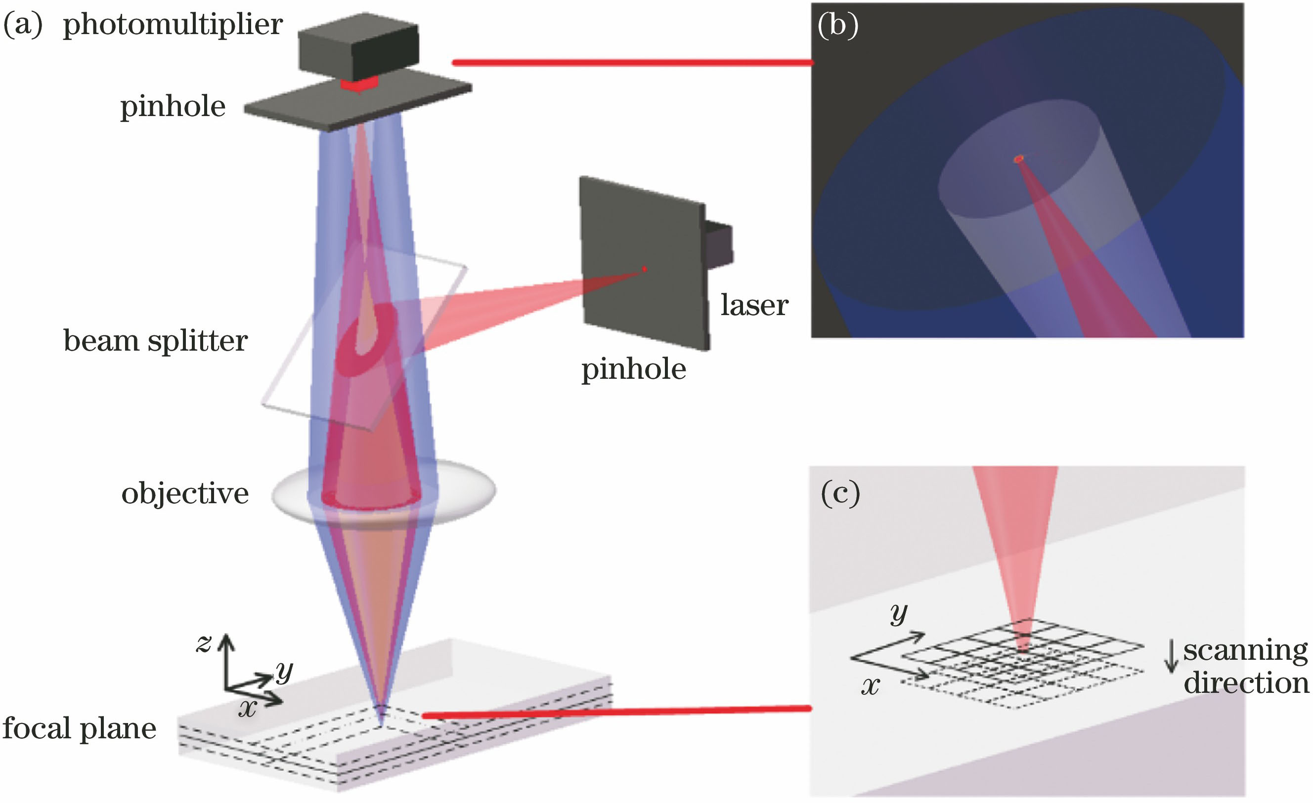
Fig. 1. Imaging principle of laser scanning confocal microscope. (a) Device principle; (b) pinhole structure; (c) horizontal and vertical scanning
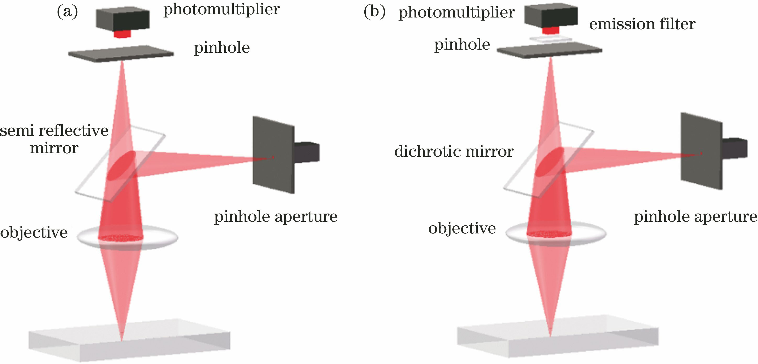
Fig. 2. Two modes of silica detected by laser scanning confocal microscope. (a) Scattering mode; (b) fluorescence mode
Fig. 3. Typical subsurface defects collected by confocal microscope. (a) Pitting defect; (b) pit defect
Fig. 4. Processing effects of Fig. 3 (b) by using defect enhancement algorithm. (a) Enhanced image; (b) aggregated image
Fig. 5. Principle of double-threshold aggregation algorithm. (a) Original image; (b) processed image
Fig. 6. Principle of improved MC algorithm based on octree algorithm. (a) Establishment of volume data; (b) octree segmentation
Fig. 7. Flow chart of three-dimensional reconstruction algorithm
Fig. 8. Reconstruction of pit defect in simulation. (a) Simulated defect; (b) reconstructed defect in simulation; (c) residual of reconstruction
Fig. 9. Tomography image obtained from simulation. (a) Cross-section of defect from simulation; (b) confocal tomography image obtained from simulation
Fig. 10. Restoration ratio of point cloud after reconstruction by three different algorithms
Fig. 11. Detection results of subsurface defects. (a) Scratch defect; (b) microcrack defect; (c) pit defect
Fig. 12. Subaperture scanning images
Fig. 13. Reconstruction results of subsurface defects. (a)(b) Reconstruction results of scratch defects; (c)(d) reconstruction results of microcrack defects; (e)(f) reconstruction results of pit defects
Fig. 14. Destructive test results of subsurface defects of fused silica. (a) Etching test results of pit defects[17]; (b) polishing-residual subsurface defects[18]; (c) scratch defects[19]; (d) pit defects[20]
| ||||||||||||||||||||||||||||||||||||||||||||||||
Table 1. Running time and occupied memory spaces of three different algorithms
|
Table 2. Defect volume distributions of experimental samples

Set citation alerts for the article
Please enter your email address
© Copyright 2018-2021 | Chinese Laser Press. All Rights Reserved 沪ICP备15018463号-20