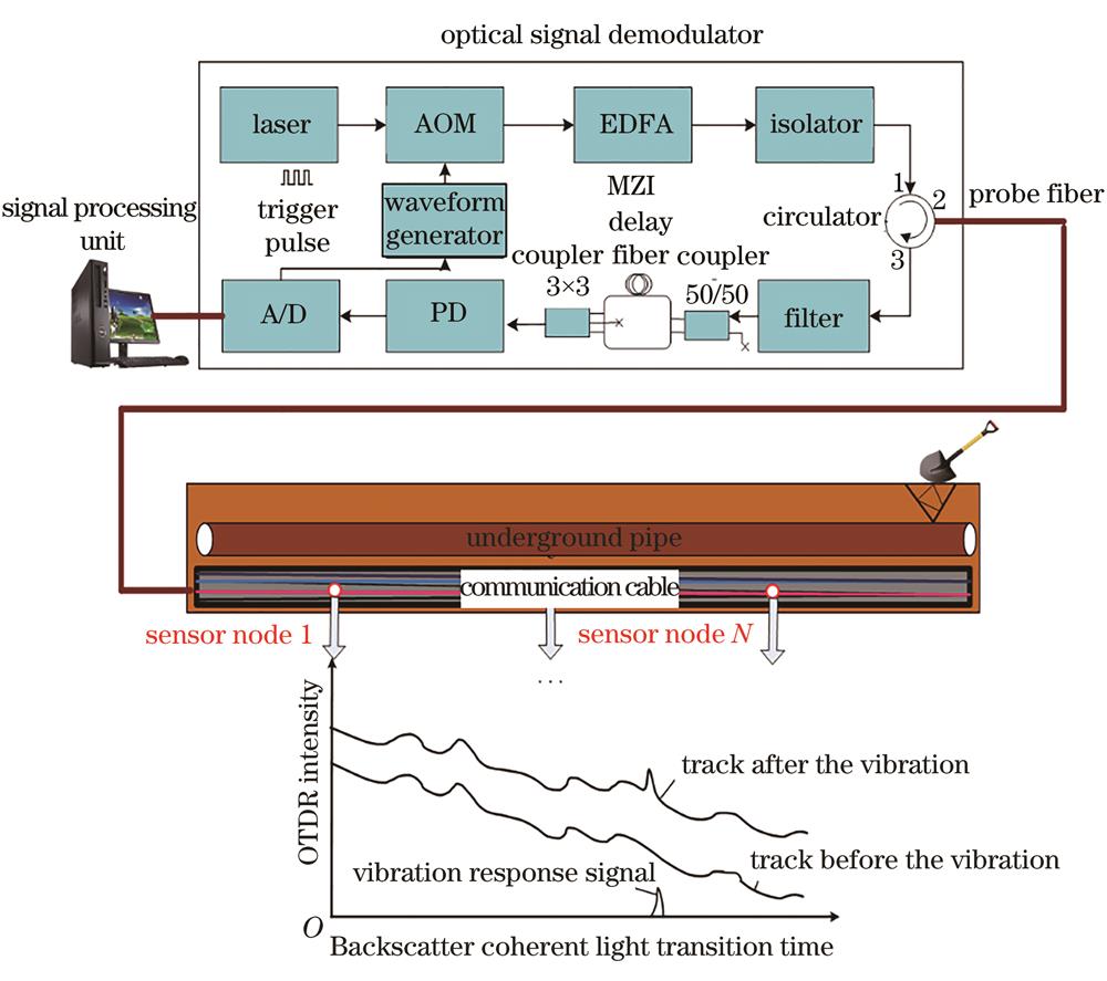
Fig. 1. Principle of the DVS/DAS based on Φ-OTDR

Fig. 2. Spatio-temporal structure of the Φ-OTDR signal^[44]

Fig. 3. De-noising and anomaly detection results based on STFT. (a) Original differential trace; (b) local energy distribution along the trace; (c) local energy distribution after the background subtraction; (d) intrusion detection and location in the energy trace; (e) intrusion detection and location in the original differential trace^[45]

Fig. 4. Signal-noise separation method based on multi-scale wavelet decomposition^[44]

Fig. 5. Signal-noise separation results based on multi-scale wavelet decomposition. (a) Original temporal signal; (b) combined component of a₆ and d₆; (c) combined component of d₃ and d₄; (d) combined component of d₁ and d₂^[44]

Fig. 6. Signal-noise separation results based on multi-scale wavelet decomposition. (a) Before the signal-noise separation; (b) after the signal-noise separation^[45]

Fig. 7. Mining and recognition processing flow of sequential information based on HMM^[36]

Fig. 8. State transition relationship between short-term SU features^[36]

Fig. 9. Common typical event signals. (a) Background noise; (b) manual digging signal; (c) machine excavation signal; (d) traffic interference; (e) forging plant noise; (f) fabricating plant noise^[36]

Fig. 10. Hidden state sequence mined by HMM. (a) Background noise; (b) manual digging signal; (c) machine excavation signal; (d) traffic interference; (e) forging plant noise; (f) fabricating plant noise^[36]

Fig. 11. Training losses of different CNNs^[33]

Fig. 12. Classification results of different CNN^[33]

Fig. 13. Classification results of 1D-CNN combined with different models^[33]

Fig. 14. Ten-fold cross classification results of 1D-CNN combined with different models^[33]

Fig. 15. Spatio-temporal feature extraction process based on CNN-BiLSTM^[42]

Fig. 16. Visualization results of different features. (a) Artificial features; (b) 2D-CNN features; (c) BiLSTM features; (d) CNN-BiLSTM features^[42]

Fig. 17. Ten-fold cross-validation results of different models^[42]

Fig. 18. Recognition time of single sample^[42]

Fig. 19. Spatial energy distribution characteristics with different vertical distances. (a) 6 m; (b) 14 m^[46]

Fig. 20. Vertical distances estimation method based on spatial energy distribution and integrated learning model^[46]

Fig. 21. Test signal of the mechanical knocking. (a) Knocking scene; (b) time domain signal diagram^[46]

Fig. 22. Spatial energy attenuation curves of the machine knocking signals. (a) Group 1; (b) group 2^[46]

Fig. 23. Test signal of the mechanical excavation. (a) Excavation scene; (b) time domain signal diagram^[46]

Fig. 24. Spatial energy attenuation curves of the excavation signals^[46]

Fig. 25. Principles of border control and security technology^[7]

Fig. 26. Laying method of optical cable and the monitoring signal before and after noise removal. (a) Laying method of the optical cable; (b) monitoring signal before denoising; (c) monitoring signal after denoising^[7]

Fig. 27. Monitoring site for excavation prevention of long-distance oil pipelines. (a) Monitoring equipment; (b) gas station; (c) on-site test environment^[49]

Fig. 28. Characteristic radar chart of typical event in an oil pipeline. (a) Background noise; (b) manual excavation; (c) mechanical excavation; (d) traffic disturbance; (e) factory interference

Fig. 29. Principle of the pipeline optical cable anti-theft and operation and maintenance monitoring system

Fig. 30. Interface of online monitoring and inspection. (a) Online positioning and inspection based on Baidu map; (b) statistical results of optical cable information

Fig. 31. Project site of submarine cable safety monitoring. (a) Monitored marine area; (b) monitoring center; (c) monitoring setup

Fig. 32. Monitoring site and test equipment of overhead transmission cables. (a) Monitoring center; (b) monitoring setup^[49]

Fig. 33. Frequency and space distribution of cable wind dance. (a) 1:00—2:00; (b) 14:00—15:00^[50]

Fig. 34. Installation wiring diagram of outdoor optical cable. (a) Sectional view; (b) top view; (c) installation process^[4]

Fig. 35. Leak response signal of the DVS/DAS system. (a) Response graph of leakage when the valve is not opened; (b) response graph of leakage when the valve is opened^[4]

Table 1. DVS/DAS signal detection and recognition method combined with machine learning model

Table 2. Actual detection results of different methods

Table 3. Local structural features of the short-term SU

Table 4. Classification performances of different models

Table 5. Parameters of CNN with different dimensions

Table 6. Model recognition results of the mechanical knock events^[46]

Table 7. Location results of the mechanical excavation^[46]