Measurement of out-of-plane deformation of curved objects with digital speckle pattern interferometry

Pengfei Li; Ping Cai; Jun Long; Chiyue Liu; Hao Yan

doi:10.3788/COL201816.111202

Abstract

Digital speckle pattern interferometry (DSPI) is a high-precision deformation measurement technique for planar objects. However, for curved objects, the three-dimensional (3D) shape information is needed in order to obtain correct deformation measurement in DSPI. Thus, combined shape and deformation measurement techniques of DSPI have been proposed. However, the current techniques are either complex in setup or complicated in operation. Furthermore, the operations of some techniques are too slow for real-time measurement. In this work, we propose a DSPI technique for both 3D shape and out-of-plane deformation measurement. Compared with current techniques, the proposed technique is simple in both setup and operation and is capable of fast deformation measurement. Theoretical analysis and experiments are performed. For a cylinder surface with an arch height of 9 mm, the error of out-of-plane deformation measurement is less than 0.15 μm. The effectiveness of the proposed scheme is verified.

Digital speckle pattern interferometry (DSPI) has proven to be a powerful tool that is widely used for the measurement of displacement/deformation^[1–6], material properties^[7], object shape^[8–12], and even temperature^[13–16]. Especially, as an interferometry-based technology, DSPI is widely recognized as a full-field, non-contact type deformation measurement technique with an accuracy of sub-micrometers^[1–6]. To measure a deformation, two DSPI interferograms are recorded before and after deformation, respectively. By image processing of the subtraction of the two interferograms, the deformation is acquired. DSPI technology has been widely applied in the measurements for planar objects. However, for objects with curved surfaces, it is difficult for DSPI to provide correct deformation measurements. This is because the sensitivity vector of deformation varies with the shape of the curved objects. In order to obtain the correct deformation of a curved surface, the shape should be known and included in the measurement. Therefore, for objects with curved surfaces, shape information and displacement information are both needed in order to obtain correct deformation measurements.

Various combinations of shape and deformation measurement techniques have been investigated by researchers in the interferometry-based deformation measurement domain. A comprehensive combination of shape and deformation measurement was proposed by Dekiff et al.^[17]. The deformation along the optical axis was measured by digital holographic interferometry (DHI), and the shape measurement is performed by stereophotogrammetry. With the shape information, the deformation was correctly measured. However, at least three CCD cameras are required in this technique, with two CCDs for shape measurement and the third CCD for deformation measurement, which makes the experiment setup complex. Another technology utilized to determine both shape and deformation was proposed by Beeck et al.^[18], where fringe projection technology combined with the phase shifting method was used for shape measurement, and holographic interferometry was adopted to measure the displacement. Because additional structure illumination and phase shifting setups are employed, the setup is also complex. Meanwhile dynamic deformation measurement is hard to achieve with the phase shifting method.

Besides the above mentioned stereophotogrammetry and fringe projection techniques, other three-dimensional (3D) shape measurement techniques, such as laser scanning, laser speckle pattern sectioning, and moire^[8–12], can also be combined with interferometry-based deformation techniques for the correct deformation measurement of curved objects. However, similar to the methods in references^[16,17], such combinations are always associated with the problem of complex setup due to the adoption of two different techniques. The DSPI technique can also be used to measure shape^[19–21]. Thus, a simpler approach was proposed by Yang et al.^[19], in which only DSPI technology was utilized for both shape and deformation measurements. Dual-beam illumination was used for the shape measurement, and single-beam illumination with phase shifting interferometry was adopted to measure the deformation. On one hand, real-time deformation measurement is hard to achieve with phase shifting interferometry. On the other hand, beam switching between shape and deformation measurements was needed in implementation, and three optical paths were built in the setup for shape and deformation measurements. All of these made the operation process complicated.

Sign up for Chinese Optics Letters TOC. Get the latest issue of Chinese Optics Letters delivered right to you！Sign up now

In this work, we propose a simple DSPI technique for both shape and fast out-of-plane deformation measurement for curved objects undergoing out-of-plane deformations. The proposed DSPI technique adopts only one single DSPI setup and one single-beam illumination. Therefore, both the setup configuration and operation are simple. The Fourier transform (FT) method is utilized to evaluate the phase from interferograms in the proposed scheme, further promoting fast performance. In the case of large field of view, where spherical wave illumination is used, however, shape measurement error is generated. An error compensation method is proposed to correct the error associated with spherical wave illumination. Theoretical analysis is performed. Experiments for the proposed scheme and the proposed error compensation method are performed. The effectiveness of the proposed scheme and method is proved.

The proposed technique includes three steps. The first step is to measure the shape of a curved object. To obtain the shape of the object, interferograms with two different illumination angles are recorded by rotating the illumination beam. The shape information is encoded in the difference of the two interferograms. By image processing, the 3D shape information is decoded. Sensitivity vectors are calculated from the 3D shape data. Secondly, the dynamic deformation along the optical axis direction is measured. Two interferograms before and after deformation are recorded. The FT method is utilized to obtain the phase difference of the interferograms and then evaluate the deformation^[18]. Finally, the true out-of-plane deformation is obtained from the measured deformations along the optical axis direction based on the sensitivity vectors of the curved object calculated in the first step.

For an object with a large size, illumination of the spherical wave is used to generate a larger illumination field. In the case of spherical wave illumination in the shape measurement in the first step, error compensation is implemented to correct the shape measurement error and, therefore, the out-of-plane deformation measurement error to improve the measurement accuracy. In the following part, the three steps are discussed in detail.

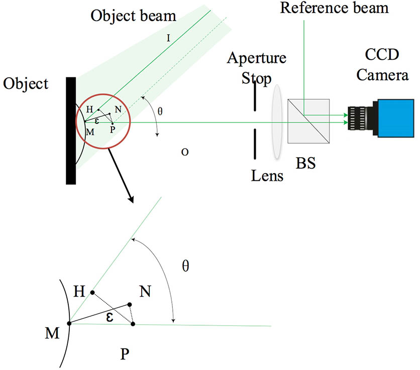
The DSPI technique has been well-applied to the deformation measurements for plane objects. Figure 1 illustrates the principle of DSPI in deformation measurement. Assuming $M$ is a point on the curved object, $IM$ denotes the illumination direction, and $MO$ denotes the observation direction, which is adjusted to be in line with the optical axis of the system.

Figure 1.Geometry of DSPI system for deformation measurement.

In this work, we consider the case that the deformation is generated mainly in the optical axis direction, while the deformation in the direction perpendicular to the optical axis is very small. In such a case, the maximum deformation is in line with the optical axis. We illustrate such a case in Fig. 1. $M$ is an arbitrary point on the object. After deformation, M moves to $P$ along the optical axis direction. A displacement $d (d = MP)$ in the optical axis direction is generated correspondingly. We denote $H$ as the foot position of common perpendicular ( $HP$ ) of two illumination beams before and after deformation. The optical path difference ( $Δ L$ ) introduced by the deformation is expressed as $Δ L = MP + MH = d (1 + \cos θ),$ (1)where $θ$ is the angle between the illumination direction and observation direction. The corresponding phase difference is $Δ Ø = 2 π Δ / λ .$ (2)

Based on Eqs. (1) and (2), the deformation d is derived as $d = \frac{λ}{2 π} \frac{Δ Ø}{1 + \cos θ},$ (3)where $λ$ is the wavelength of the illumination beam. The out-of-plane deformation $d_{n} = MN$ is $d_{n} = \frac{λ}{2 π} \frac{Δ Ø \cos ε}{(1 + \cos θ)},$ (4)where $ε$ represents the angle between the normal vectors (in the MN direction) of the curved surface and optical axis (in the MO direction).

In Eq. (4), parameters $λ$ and $θ$ are known system parameters, but parameters $Δ Ø$ and $ε$ are unknown. Parameter $ε$ depends on the 3D shape of the object and is not a constant when the object has a curved surface. That is to say, $ε$ varies point by point on the curved surface. Therefore, in order to obtain the out-of-plane deformation $d_{n}$ in Eq. (4), the 3D shape of the curved surface must be obtained first. In the DSPI technique, the phase difference $Δ Ø$ in Eq. (4) is obtained by processing the subtraction of the two interferograms recorded before and after deformations, which will be discussed in the next section.

In both the shape and deformation measurements of the proposed schemes, two interferograms are recorded. The shape and the deformation information are all decoded in the phase difference ( $Δ Ø$ ) of the two interferograms. Therefore, how to determine $Δ Ø$ from the two interferograms is a key issue. In this work, the FT approach^[22–27] is adopted. Other methods also exist, such as the phase shifting method. The advantage of the FT method is fast calculation and the avoidance of using a piezoelectric transducer (PZT) in the system, as in the phase shifting approach, such that real-time phase evaluation is possible.

The phase evaluation process is discussed below. In order to separate the spectrum, an angle was implemented between the reference and object waves, resulting in a spatial carrier^[27]. For the intensity of a recorded interferogram, where the interference between the object wave and reference wave can be expressed as $i (x, y) = a (x, y) + b (x, y) \cos [δ (x, y) + 2 π f_{x} x + 2 π f_{y} y],$ (5)where $f_{x}$ and $f_{y}$ are the spatial carrier frequency in the $x$ and $y$ directions, $δ (x, y)$ is the phase of the interferogram. Equation (5) can also be expressed as^[28] $i (x, y) = a (x, y) + c (x, y) [\exp (2 π f_{x} x i) + \exp (2 π f_{y} y i)] + c^{*} (x, y) [\exp (- 2 π f x i) + \exp (- 2 π f_{y} y i)],$ (6)where $c (x, y)$ is $c (x, y) = \frac{1}{2} b (x, y) \exp [δ (x, y) i],$ (7)and $*$ represents the complex conjugate. Performing two-dimensional FT to Fig. 2(a) by Eq. (6), the intensity is transformed into the Fourier domain. Figure 2(b) shows an example of the intensity of Eq. (8) in the Fourier domain. The spectrum of the interferogram in the Fourier domain is $I ({f f}_{x}, {f f}_{y}) = A ({f f}_{x}, {f f}_{y}) + C^{*} ({f f}_{x} - f_{x}, {f f}_{y} - f_{y}) + C^{*} ({f f}_{x} + f_{x}, {f f}_{y} + f_{y}),$ (8)where ${f f}_{x}$ and ${f f}_{y}$ represent the coordinates of the $x$ and $y$ axis, respectively, in the Fourier domain. The term $A ({f f}_{x}, {f f}_{y})$ located in the center of the Fourier domain is the zero order term, which comes from background information. Terms $C ({f f}_{x} - f_{x}, {f f}_{y} - f_{y})$ and $C^{*} ({f f}_{x} + f_{x}, {f f}_{y} + f_{y})$ , which are centrally and symmetrically distributed with respect to the origin, are the two first orders representing the object information. In the processing, $C ({f f}_{x} - f_{x}, {f f}_{y} - f_{y})$ or $C^{*} ({f f}_{x} + f_{x}, {f f}_{y} + f_{y})$ is filtered out and shifted to the center of the Fourier domain, such that $C ({f f}_{x}, {f f}_{y})$ or $C^{*} ({f f}_{x}, {f f}_{y})$ , which is the spectrum of $c (x, y)$ in Eq. (6) or its conjugate, is obtained in the Fourier domain. The $c (x, y)$ in Eq. (6) is calculated by applying an inverse two-dimensional FT to $C ({f f}_{x} - f_{x}, {f f}_{y} - f_{y})$ or $C^{*} ({f f}_{x} + f_{x}, {f f}_{y} + f_{y})$ . The phase of $c (x, y)$ is calculated as^[23–25] $Ø (x, y) = \frac{Im [c (x, y)]}{R e [c (x, y)]} .$ (9)

Figure 2.Illustration of the phase evaluation process. (a) DSPI interferogram. (b) Spectrum of an interferogram in the Fourier domain. (c) The wrapped phase difference $Δ Ø$ . (d) The unwrapped continuous phase difference $Δ Ø$ .

Equations (6) to (9) explain how the phase of an interferogram is obtained. The phase difference $Δ Ø$ between two interferograms can be calculated as $Δ Ø (x, y) = \frac{Im [c_{1} (x, y) \times c_{2}^{*} (x, y)]}{R e [c_{1} (x, y) \times c_{2}^{*} (x, y)]},$ (10)where $c_{1}$ and $c_{2}$ represent $c (x, y)$ of the two interferograms. The wrapped phase difference $Δ Ø (x, y)$ is presented in Fig. 2(b) as an example. The short-time FT filter is performed to reduce the noise in the wrapped phase fringe pattern^[29]. Finally, phase unwrapping is implemented to transform the fringe pattern to continuous form of $Δ Ø (x, y)$ ^[30], which is shown in Fig. 2(c).

We adopt the single-beam DSPI configuration in shape measurement, as shown in Fig. 3, instead of the dual-beam configuration^[18]. The same single-beam DSPI configuration is used in the deformation measurement, which makes the optics setup simple. As in Fig. 2, $θ$ is the illumination angle. The illumination beam is rotated by $Δ θ$ from $MI$ to ${MI}^{'}$ , which can be assumed that point source $I$ at infinity was translated to $I^{'}$ . The optical path difference ( $Δ L$ ) is generated due to the rotation of the illumination angle^[9]. The corresponding phase difference $Δ Ø$ at an arbitrary point $M (x, y, z)$ can be described as $Δ Ø = \frac{2 π Δ L}{λ} = \frac{2 π (M I - M I^{'})}{λ} .$ (11)

Figure 3.Geometry of DSPI system for shape measurement.

The initial position of the light source $I$ at infinity can be assumed to be the origin of the coordinate system. $I^{'} (x_{1}, y_{1}, z_{1})$ denotes the light source position after beam rotation. Because the rotation angle $Δ θ$ is very small, the optical path difference $Δ L$ is formulated as^[10] $Δ L = \sqrt{{(x - x_{1})}^{2} + {(y - y_{1})}^{2} + {(z - z_{1})}^{2}} - \sqrt{x^{2} + y^{2} + z^{2}} \approx \frac{{x x}_{1} + {y y}_{1} + {z z}_{1}}{\sqrt{x^{2} + y^{2} + z^{2}}} .$ (12)

The deflection of the illumination beam is in the x‐z plane, such that $y_{1} = 0$ , and $x_{1}$ and $z_{1}$ can be denoted as^[22] $x_{1} = x Δ θ, z_{1} = z Δ θ .$ (13)

$Δ L$ can be simplified as $Δ L = (z \sin θ + x \cos θ) Δ θ,$ (14)where $\sin θ$ and $\cos θ$ are $\sin θ = \frac{x}{\sqrt{x^{2} + y^{2} + z^{2}}}, \cos θ = \frac{z}{\sqrt{x^{2} + y^{2} + z^{2}}} .$ (15)

Combining Eqs. (11) and (15), the height $z$ is obtained as $z = \frac{Δ Ø λ}{2 π \sin θ Δ θ} - \frac{x}{\tan θ Δ θ} .$ (16)

The shape of the object can be described as $F (x, y, z) = \frac{Δ Ø λ}{2 π \sin θ Δ θ} - \frac{x}{\tan θ Δ θ} - z = 0.$ (17)

Then, the normal vector is $n_{0} = {\frac{\partial F}{\partial x}, \frac{\partial F}{\partial y}, \frac{\partial F}{\partial z}}$ . Consider that the unit vector of the optical axis direction is $n_{op} = {0, 0, 1}$ . $ε$ can be obtained as $ε = \arccos 〈 n_{0}, n_{op} 〉 .$ (18)

In the shape measurement, the angle $θ$ is used to adjust the sensitivity of the optical path length measurement in the lateral and axis directions. The angle between 40° and 50° is preferred^[8].

When the illumination beam is a spherical wave, $θ$ is not a constant over the whole CCD field. The larger the field size is, the larger the error of the illumination angle will be. A widely adopted method to control the error is to keep the ratio of the object distance to the size of object much larger than 1^[9,22], such that the non-collimation effect is not severe. Although such a method can control the error caused by the spherical wave illumination to a certain extent, the error still exists and affects the measurement accuracy, especially for high-precision measurement.

In this work, the illumination angle $θ_{0}$ is assumed to arrive at the object at central point $M_{0} (x_{0}, y_{0}, z_{0})$ of the object, which is determined by the physical structure. Due to $x$ and $y$ also being expressed by the numbers of the pixel size, Eq. (15) can be represented by $\sin θ_{(x_{m}, y_{n})} = \frac{x_{0} + mu}{\sqrt{{(x_{0} + mu)}^{2} + {(y_{0} + nu)}^{2} + z_{0}^{2}}}, \cos θ_{(x_{m}, y_{n})} = \frac{z_{0}}{\sqrt{{(x_{0} + mu)}^{2} + {(y_{0} + nu)}^{2} + z_{0}^{2}}},$ (19)where $u$ represents the enlarged pixel size, $m$ and $n$ are pixel indexes in the $x$ and $y$ directions with respect to $x_{0}$ and $y_{0}$ , and $θ_{(x_{m}, y_{n})}$ represents the illumination angle at each pixel $(x_{m}, y_{n})$ .

In Eq. (19), while the values of $x_{0}$ and $y_{0}$ are much larger than the size of the measurement field, $θ$ is assumed to be a constant equal to $θ_{0}$ . But for a large size field, $θ$ is a function of $x$ and y. The error of the spherical wave illumination is $e = \frac{Δ Ø λ}{2 π [\sin θ_{0} - \sin θ_{(x_{m}, y_{n})}] Δ θ} - \frac{x}{[\tan θ_{0} - \sin θ_{(x_{m}, y_{n})}] Δ θ} .$ (20)

Assume that the size of the field of view is $100 mm \times 100 mm$ , the object distance is 500 mm, and the maximal angle difference in the field is 8.4 and results in the maximum error of 0.925 mm at the edge for the shape height of 9 mm, which should not be ignored for shape measurement.

The DSPI setup is shown in Fig. 4. A semiconductor laser with a wavelength of 532 nm and power of 50 mW is used as the light source. A beam expander (BE1) transforms a point light source to a plane wave and expands the beam by five times. By splitting the parallel beam into two beams by a polarizing beam splitter (PBS), the object wave and reference wave are generated. Another beam expander (BE2) located between the object and mirror 1 further expands the parallel reference beam to a larger field (five times more than before) of illumination. Two half-wave plates (HWP1, HWP2) in combination with the PBS are used to adjust the intensity ratio between the object beam and reference beam for better interferogram quality. The object beam reflected by the object surface is collected by an imaging lens, which generates a reduced image of the object at the CCD camera (DMK 51BU02) with $1600 p i x e l \times 1200 p i x e l .$ The pixel size is 4.65 μm. The imaging lens has a focal length of 85 mm and shrinks the field of view by 10 times, such that a larger field of view of $50 mm \times 37.5 mm$ is finally recorded by the CCD. An aperture slot is used before the imaging lens to reduce the high-frequency noise and improve the interference quality.

Figure 4.Experimental DSPI setup.

In this work, two experiments are performed. In one experiment, the spherical wave illumination surface profiling is implemented, and the compensation effect of the proposed method is evaluated. In the other experiment, the proposed DSPI technique for out-of-plane deformation measurements of a curved object is examined.

A 3D printed cylinder surface with arch height of 9 mm is used as the test piece. A pitching stage is employed to introduce displacement along the optical axis. Firstly, the shape measurement is performed. Mirror 1 mounted in a rotation stage (TTR001/M, Thorlabs) rotates the illumination beam by an angle of $Δ θ = 0.03 °$ . The CCD camera records two interferograms before and after beam deflection. The shape data is then calculated by Eq. (16), and shape-related parameter $ε$ is calculated by Eq. (18). Secondly, the object is displaced in the direction of optical axis. With one edge fixed, the other parallel edge is displaced. The applied rotation angle changes from 0° to 0.0515° with an interval of 0.00515°. The CCD camera records the interferograms before and after the displacements. The deformations along the optical axis direction are calculated with Eq. (3). Combining the results of shape data, the out-of-plane deformations can be calculated by Eq. (4).

Firstly, shape measurement is implemented. The measurement result of a cylinder surface of an arch height of 9 mm is shown in Fig. 5. The 3D shape is shown in Fig. 5(a). A section in the center of the surface is shown in Fig. 5(b). Figure 5(c) shows the normal vector $n_{0}$ of the curved surface to calculate $ε$ . The measured value of the arch is 9.24 mm. Taking into account the error of 3D printing that is 0.05 to 0.4 mm, the shape measurement error from the design value of 9 mm is relatively small and acceptable.

Figure 5.Experiment result of out-of-plane deformation measurement for curved objects. (a) The wrapped phase difference $Δ Ø$ . (b) The unwrapped continuous phase difference $Δ Ø$ . (c) Shape measurement result. (d) A section through the center of the surface.

Figure 6.Experiment result of deformation measurement for a cylinder surface. (a) The wrapped phase difference $Δ Ø$ . (b) The unwrapped continuous phase difference $Δ Ø$ . (c) The measured deformation in the direction of optical axis. (d) An example of out-of-plane deformation of cylinder surface. (e) The measured and applied rotation angles in the optical axis direction. (f) Comparison between the measured and theoretical applied out-of-plane deformation in the $x$ axis. (g) Comparison between the measured and theoretical applied out-of-plane deformation in the $y$ axis. (h) The MSEs of the measured out-of-plane deformations in the whole field of view for the 10 different loads (indexed by case number).

Secondly, the deformation measurement is implemented after shape measurement. The displacement of a rigid body is used to substitute the deformation in this experiment. The displacement is implemented in the direction of the optical axis with an interval of 10 μm by a differential micrometer drive. The experimental measurement results are compared with theoretical values, as shown in Fig. 6. Figure 6(a) shows the deformation measured along the optical axis direction. From the measured deformations in the optical axis direction in Fig. 6(a), the applied rotation angles are derived and compared with the true applied rotation angles in Fig. 6(c). The measured deformations and the applied deformations agree well with each other. The 3D out-of-plane displacement of the curved surface is further calculated by including the measured 3D shape in Fig. 5(a), and the result is presented in Fig. 6(b). The profiles of the 3D out-of-plane displacement in Fig. 6(b) in the $x$ and $y$ directions are shown in Figs. 6(d) and 6(e), respectively, where the measurement results are compared with the theoretical applied values. The mean square errors (MSEs) between the measured out-of-plane deformations and the theoretical applied out-of-plane deformations are calculated in the whole field of view for 10 loads, and the result is shown in Fig. 6(f). It is seen that the MSE is from about 0.06 to 0.093 μm, which indicates that the proposed out-of-plane deformation measurement technique for a curved object has high accuracy. The effectiveness of the proposed technique is verified.

To evaluate the proposed compensation method for reduction of the error caused by the spherical wave illumination, the shape measurement experiment is implemented with spherical wave illumination, and the compensation methods in Eqs. (19) and (20) are applied to the measurement. The results are shown in Fig. 7.

Figure 7.Experiment result of 3D shape measurement with spherical wave illumination. (a) 3D shape measurement with spherical wave illumination after compensation. (b) Comparison between the results with and without compensation in the $x$ axis. (c) The MSE with and without compensation.

The experimental results show that the MSE caused by the spherical wave illumination is reduced by about 50% with the proposed compensation method. Hence, the effectiveness of the proposed method is verified. We recommend using such a compensation method in spherical wave illumination, especially for objects with larger size, to improve the measurement accuracy in both shape and further the out-of-plane deformation.

A methodology for 3D shape and out-of-plane deformation measurement of curved objects with only one single DSPI setup and one illumination beam is proposed. Compared to current interferometry-based techniques for out-of-plane deformation measurement of curved objects, the proposed technique is simpler in both setup and operation and allows fast measurement. The preliminary experiments are performed, and the effectiveness of the proposed technique is verified with a high accuracy.

References

[1] L. Yang, X. Xie, L. Zhu, S. Wu, Y. Wang. Chin. J. Mech. Eng., 10, 3901(2014).

[2] R. Kulkarni, P. Rastogi. Opt. Lasers Eng., 87, 1(2016).

[3] P. K. Rastogi. Digital Speckle Pattern Interferometry & Related Techniques, 384(2000).

[4] G. Pedrini, J. Gaspar, O. Paul, W. Osten. Chin. Opt. Lett., 7, 1109(2009).

[5] P. Sun, R. Liu, Q. Han, X. Wang. Chin. Opt. Lett., 4, 709(2006).

[6] L. Xia, M. Guan, X. Sang, X. Cao, Z. Chen. Chin. Opt. Lett., 15, 120901(2017).

[7] M. Kumar, G. S. Khan, C. Shakher, 9660, 966011(2015).

[8] F. Chen, G. M. Brown, M. Song. Opt. Eng., 39, 10(2000).

[9] C. Song, A. S. G. Prasad, K. H. Chan, V. M. Murukeshan. Rev. Sci. Instrum., 87, 063116(2016).

[10] R. Rodriguez-Vera, D. Kerr, F. Mendoza-Santoyo. J. Opt. Soc. Am. A, 9, 2000(1992).

[11] R. M. Groves, S. W. James, R. P. Tatam. Opt. Lasers. Eng., 41, 621(2004).