
Han Bai, Yun Yang, Qinfang Cui, Peng Jia, Lixia Wang. Retrieval of Heavy Metal Content in Soil Using GF-5 Satellite Images Based on GA-XGBoost Model[J]. Laser & Optoelectronics Progress, 2022, 59(12): 1230001
- Laser & Optoelectronics Progress
- Vol. 59, Issue 12, 1230001 (2022)
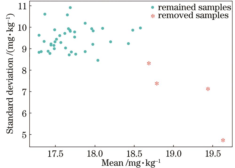
Fig. 1. Mean-standard deviation distribution of MCCV method
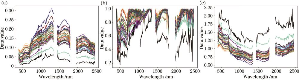
Fig. 2. Spectral curves of different kinds of spectral transformations. (a) R; (b) CR; (c) log R-1
Fig. 3. Correlation analysis of different spectral transformations and heavy metal content
Fig. 4. Scatter diagrams of prediction results of CFS-XGBoost. (a) R; (b) log R-1; (c) CR
Fig. 5. Scatter diagram of prediction results of GA-XGBoost. (a) R; (b) log R-1; (c) CR
Fig. 6. Results of correlation coefficient feature selection and GA feature selection
Fig. 7. Feature importance scores given by XGBoost
Fig. 8. Spatial distribution of Cu content
|
Table 1. Comparison of hyperspectral satellite parameters
|
Table 2. Comparison between measured Cu content and regional background value
|
Table 3. Statistics of correlation coefficient between original spectrum and its two transformations with Cu content
|
Table 4. Statistical characteristics of training set and testing set
| |||||||||||||||||||||||||||||||||||||||||||||||||||||||||||||||||
Table 5. Precision comparison of XGBoost model based on GA and CFS feature selection methods
|
Table 6. Statistics of copper content estimation results

Set citation alerts for the article
Please enter your email address
© Copyright 2018-2021 | Chinese Laser Press. All Rights Reserved 沪ICP备15018463号-20