Fig. 1. (a) Shows the effects of CEP on the electric field and the intensity of the wave. The red line is a sine waveform and the blue line is a cosine waveform. $E(t)$ is the electric field of the light, $a(t)$ is the Gaussian intensity envelope of the function, $\unicode[STIX]{x1D719}$ is the CEP as defined in Equation (3). (b) Shows the intensity $I(t)$ of the sine and cosine laser pulses. $\unicode[STIX]{x1D6FF}_{CEP}$ is defined as being the difference in peak intensity between the two waveforms, as shown.

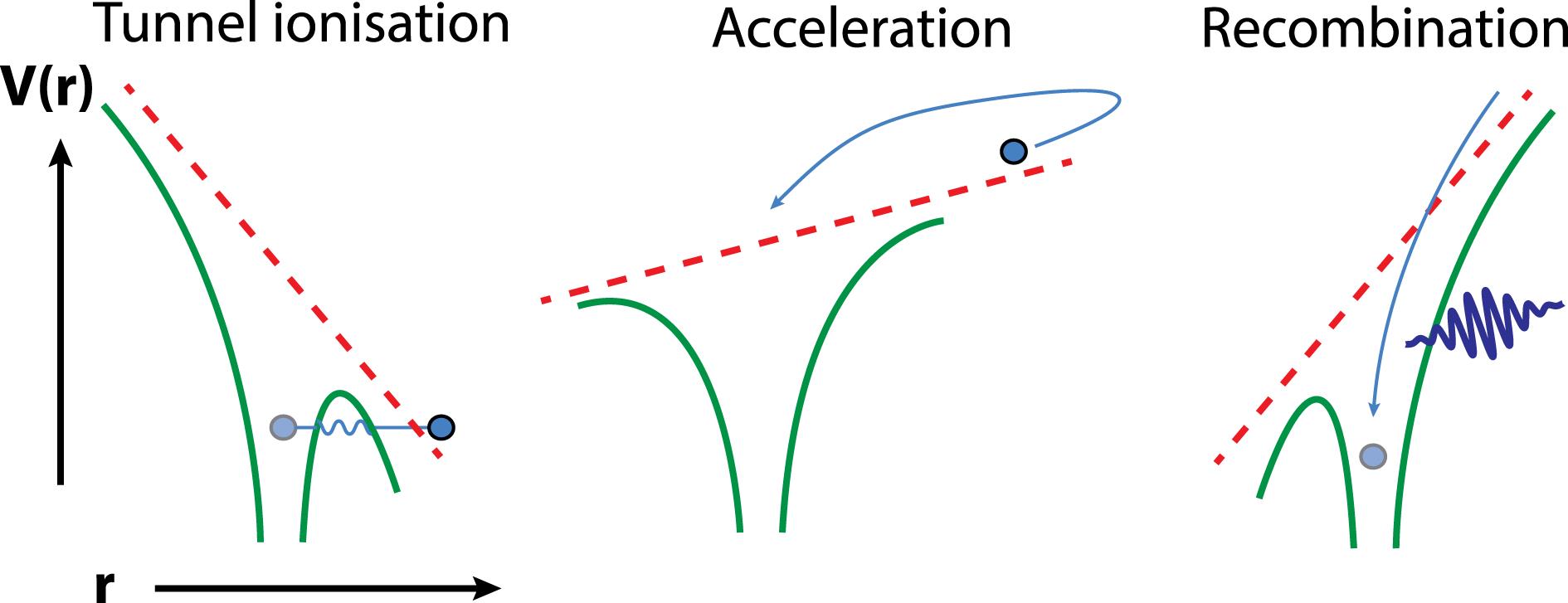
Fig. 2. A diagrammatic representation of the three-step model. $V(r)$ is the atomic potential, $r$ is the radial distance from the atomic core. In the first step, the atomic potential (green line) is suppressed by the laser field (red dashed line), to the point where the valence electron (grey sphere) can tunnel into free space. The second step is acceleration of the electron by the laser field. The oscillating motion of the field accelerates the electron back towards the ionic core. The final stage is recombination of the electron with the ionic core. The recombination causes HHG, represented by the purple XUV photon. Recombination may also cause secondary ionization effects. If the driving laser field is not linearly ionized, recombination may not occur, in which case ATI electrons can be detected.

Fig. 3. A diagram outlining the major difference between tunnelling ionization and OBI. (a) Tunnel ionization. The electric field of the laser (red dotted line) suppresses the atomic potential binding the electron to the atomic core (blue solid line). As one side of the potential well is lowered, the probability for the valence electron to tunnel through the barrier into the continuum increases, and if the electric field is maintained at the required amplitude, over time the probability of tunnel ionization becomes unity. (b) OBI. The amplitude of the electric field is enough to suppress the potential to the point where the electron is promoted ‘over the barrier’ into the continuum.

Fig. 4. A schematic diagram of an MCP. (a) Shows the whole MCP, consisting of several single channel electron multipliers in a substrate. (b) Indicates the electron multiplication process of a single channel. A single electron generates an output electron bunch via cascading secondary emission. The voltage provides electrons to replenish those lost to free space via the secondary emission.

Fig. 5. LS coupled energy levels of the neon atom. The red state is the ground state, the two blue states are metastable states with no allowable optical transitions to lower states, and the green states are excited states with allowable optical transitions to lower states. The $^{3}P_{2}$ state is the metastable state used in this work.

Fig. 6. Figure adapted from Huismans et al.^[93]. This diagram outlines the concept of electron wavepacket holography. The electron wavepacket expanding along path I has a given momentum defined by $k_{z}$ and $k_{r}$. This is the reference wave. The electron wavepacket expanding along path II has the same defined momentum, but has scattered off the parent ion. This is the signal wave. As the wavepackets are coherent with each other, they can interfere and information about the phase difference can be obtained from observational data as per $\unicode[STIX]{x1D6E5}\unicode[STIX]{x1D711}=(k-k_{z})z_{0}$.

Fig. 7. Figure adapted from Huismans et al.^[93]. These are observations of electron momentum observed in the experiment of Huismans et al. with laser intensities as follows (all units are $\text{W}~\text{cm}^{-2}$). (A) $7.1\times 10^{11}$; (B) $5.5\times 10^{11}$; (C) $4.5\times 10^{11}$; (D) $3.2\times 10^{11}$; (E) $2.5\times 10^{11}$; (F) $1.5\times 10^{11}$. Note the side lobes that run parallel to the direction of polarization of the ionizing laser in image A have disappeared by the time the intensity has reached image F.

Fig. 8. Figure adapted from Huismans et al.^[93]. A comparison of experimentally observed results and calculated results based on both solving the TDSE and using a CCSFA approach. (A) Experimental results. (B) TDSE results. (C) SFA results. The observed side lobes are predicted by both theories. The inset on (C) is a calculation run for a half-cycle calculation, showing the lobes are a result of interference between two trajectories that leave the parent atom in the same half-cycle.

Fig. 9. Comparison between the ionization fraction of neon for a laser pulse with a peak intensity of $1.2\times 10^{13}~\text{W}~\text{cm}^{-2}$ and the electric field of the laser pulse. The ionization fraction naturally increases as the pulse passes by the atom.

Fig. 10. A measurement of the atomic beam width in the COLTRIMS for the experiments performed by Calvert et al. This was measured by scanning the ionizing laser in the $r$ direction as defined in Figure 11 and recording the ion yield. The Gaussian fit follows the equation $f(x)=a\times \exp [-(x-b)^{2}/c^{2}]$ where $a=(4.05\pm 0.40)\times 10^{4}$, $b=8.6\pm 0.1$ and $c=0.59\pm 0.07$. It has a $R^{2}=0.96$. It is clear that the Gaussian fit is not ideal, but provides a good estimation of the width of the function at the FWHM. Given that the ion yield function should be a convolution of the cylindrical atomic beam and the Gaussian laser beam, and noting the flat top of the data points, it is proposed for modelling purposes that we treat this 2D projection of the atomic beam width as a top-hat function with a width given by the FWHM of the Gaussian function of $z_{abeam}=1.39\pm 0.16$ mm. Assuming cylindrical symmetry, this flat top translates to a cylindrical atomic beam. Given the transverse velocity distribution of the atoms out of the source is assumed to be Gaussian, it might be surprising that the atom beam measurements appear to be more flat top. This is attributed to the optical collimation applied to beam.

Fig. 11. A conceptual layout of the interaction region as it was modelled for theoretical ion yield predictions.

Fig. 12. The modelling of the 2D ionization fraction map with the following laser parameters: $I_{pk}=9.6\times 10^{13}~\text{W}~\text{cm}^{-2}$; $w_{0}=7.25~\unicode[STIX]{x03BC}\text{m}$; pulse length $=$ 6.3 fs. (a) Shows the calculated points, while (b) shows the interpolated map. Both maps come from the same modelling data; however, only the interpolated map was used for further processing.

Fig. 13. An example of the total ion yield modelling output $\unicode[STIX]{x1D6FC}\left(r,z\right)$. The modelling parameters are the same as used in Figure 12. There is an area of high ionization at the centre of the focus. This is expected, as this is the location of the peak electric field. The increasing width of interaction in the $r$ direction at the extremes of the $z$ values is due to the volume effects at the edges of the Gaussian pulse, i.e., the width of the pulse increases and still has an electric field high enough in these regions to cause ionization. This is typical of systems with a low ionization potential and a laser beam Rayleigh range of the same order of magnitude as the atomic beam. As the integration across $r$ is performed as a sum of small cylindrical shell volume elements, values close to $r=0$ have a low ionization yield due to their smaller volume elements when compared to greater values of $r$. This manifests as the almost linear slope increase in ion yield up to $r\sim 30$ across all values of $z$. After that value of $r$, the ion yield probability drops due to the lower electric field amplitude at those values of $r$, and the integration effects on increasing ion yield are reduced.

Fig. 14. A comparison between the predicted ion yields for differing theoretical predictions for ionization probability of $\text{Ne}^{\ast }$ using a high intensity laser pulse. This data is modelled with the following parameters; $1.2\times 10^{6}$ pulses; pulse length of 6.3 fs; laser beam waist of $7.25~\unicode[STIX]{x03BC}\text{m}$; central wavelength of 760 nm; atomic beam flux of $1.43\times 10^{14}$ atoms/str/s. The data has been normalized.

Fig. 15. Figure adapted from Calvert et al.^[101]. Fine structure transitions for the cooling transition in neon. The $\,^{3}\text{P}_{2}$ is the metastable state. The figure shows optically allowed transitions and the squared Clebsch–Gordan coefficients for the $J=2$ to $J=3$ fine state transitions.

Fig. 16. Figure adapted from Calvert et al.^[101]. Population fraction of $m_{j}$ sublevels in $\text{Ne}^{\ast }$ atoms being pumped by $\unicode[STIX]{x1D70E}^{-}$ circularly polarized light with the parameters given in Table 1. The stretched $m_{j}=-2$ state reaches 99% population after $0.63~\unicode[STIX]{x03BC}\text{s}$. For $\unicode[STIX]{x1D70E}^{+}$ pump light, the plot is similar except with the signs of the $m_{j}$ states reversed.

Fig. 17. Figure adapted from Calvert et al.^[101]. The modelled change in the $m_{j}$ state fraction of a $\,^{3}\text{P}_{2}$ Ne atom beam as the fast axis of a quarter-wave plate is rotated around the pass axis of a linear polarizer. For clarity, only the $m_{j}=\pm 2$ states are displayed.

Fig. 18. Figure adapted from Calvert et al.^[101]. A schematic diagram of the experimental setup used by Calvert et al.^[101]. Few-cycle laser pulses are generated by the Femtopower Compact Pro CE Phase laser. Pulse lengths are controlled by the DCM’s and wedges. The half waveplate, germanium plates and flip-in pellicles are used to the optical power. The quarter waveplate is used to calibrate the peak intensity of the laser^[110]. Metastable atoms are provided by the DC discharge source, then optically collimated to increase the target flux. Only one pair of mirrors for the optical collimator is shown, whereas two pairs are employed in the actual experiment to collimate in two directions. The optical pump laser is propagating in the same direction as the electric field of the ionizing laser, which defines the quantization axis. COLTRIMS results were recorded and raw $m/q$ spectra were obtained, and example of fwhich is given in Figure 19.

Fig. 19. Typical $m/q$ spectrum. Main figure: The $m/q$ spectrum observed by the COLTRIMS with the $\text{Ne}^{\ast }$ discharge source on. Note the contaminants that exist in the vacuum chamber. Inset: m/q spectrum after background subtraction, which removes the contaminant signals, and source discharge off signal subtraction, which removes the ground-state Ne signal. The inset data is used for further analysis. The following laser parameters were used in this image: $I_{pk}=2.42\times 10^{14}~\text{W}~\text{cm}^{-2}$, $w_{0}=7.25~\unicode[STIX]{x03BC}\text{m}$.

Fig. 20. Figure adapted from Calvert et al.^[101]. Comparison of experimental data with scaled theoretical ADK and TDSE data. The theory was fit using the spline fitting described by Equation (39), and provides the following fitting coefficients for ADK theory: $A=0.29$ and $\unicode[STIX]{x1D702}=2.67$. For this fit $\unicode[STIX]{x1D712}^{2}=0.28$. For the theoretical TDSE data fit, the fitting coefficients are: $A=0.42$ and $\unicode[STIX]{x1D702}=1.59$. For this fit $\unicode[STIX]{x1D712}^{2}=0.25$.

Fig. 21. Figure adapted from Calvert et al.^[101]. Results for the ionization of $\text{Ne}^{\ast }$ while altering the fast axis of the quarter-wave plates with respect to the pass axis of a linear polarizer that are used to prepare the ellipticity of the pump light. The pump laser intensity is $(9.2\pm 4.5)\times 10^{13}~\text{W}~\text{cm}^{-2}$. The waveplate angles of circularly polarized light are indicated.

Fig. 22. Coulomb focusing in the transverse direction. (a) defines the axes, with the Poynting vector of the laser pulse travelling in the $y$ direction, and the electric field oscillating in the $x$ direction. (b) shows an electron released from its parent ion. In this case there is a small component of initial transverse momentum imparted by the ionization process; however, the large majority of the total electron momentum is in the parallel direction due to the electron being driven by the electric field. (c) occurs after a period of time as the reversal of the electric field drives the electron back past the ion. The attractive Coulomb force in the transverse direction draws the electron towards the ionic core, imparting momentum in the transverse direction. The interaction is symmetric with regards to the electric field of the light and hence leads to the focusing effect. While the exact effects of the Coulomb force vary on a pulse by pulse basis, on average there is a loss of transverse momentum as the electron is attracted to the ionic core.

Fig. 23. A definition of $\vec{p}_{trans}\equiv \vec{p}_{\bot }$ in the ionization region. The laser pulse is travelling along the $y$ direction, and as the electric field is oscillating along the $x$ direction, the plane of polarization is the $x{-}y$ plane. $\vec{p}_{\Vert }$ is in the $x$ direction and the major contribution is the electric field of the laser pulse. The direction of $\vec{p}_{\bot }$ is in the $z$ direction.

Fig. 24. Figure adapted from Ivanov et al.^[114]. TEMD of Ar for (a) $\unicode[STIX]{x1D700}=0$, (b) $\unicode[STIX]{x1D700}=0.42$ and (c) $\unicode[STIX]{x1D700}=1$, respectively. The peak laser intensity is measured to be $(4.8\pm 2.4)\times 10^{14}~\text{W}~\text{cm}^{-2}$. Theoretical data is shown as the red curve, experimental data is plotted.

Fig. 25. Figure adapted from Ivanov et al.^[114]. TEMD of $\text{Ne}^{\ast }$ for (a) $\unicode[STIX]{x1D700}=0$, (b) $\unicode[STIX]{x1D700}=0.42$ and (c) $\unicode[STIX]{x1D700}=1$, respectively. The peak laser intensity is measured to be $(2.0\pm 1.0)\times 10^{14}~\text{W}~\text{cm}^{-2}$. Theoretical data is shown as the blue curve, experimental data is plotted.

Fig. 26. A plot of electron yield as a function total electron momentum $p_{r}$. The blue line indicates the cutoff momentum above which the ionized electrons could have only undergone OBI according to Equation (40).

Fig. 27. Figure adapted from Ivanov et al.^[114]. The fitting parameter $\unicode[STIX]{x1D6FC}$ as a function of $\unicode[STIX]{x1D700}$ for both (a) Ar and (b) $\text{Ne}^{\ast }$. The square markers are TDSE data, with lines drawn in as a guide for the eyes. The circular markers are the experimental data.

Fig. 28. Calculated angular momentum distribution $N_{\ell }$ for (a) Ar and (b) $\text{Ne}^{\ast }$, with $\unicode[STIX]{x1D700}=1$. The laser intensity is $4.2\times 10^{14}~\text{W}~\text{cm}^{-2}$ for Ar ionization, which is in the tunnelling regime. The laser intensity is $2.0\times 10^{14}~\text{W}~\text{cm}^{-2}$ for $\text{Ne}^{\ast }$, which is in the OBI regime. The results indicate that with circularly polarized light, Ar atoms are shifted to higher values of $\ell$ and hence have higher orbital angular momentum impacted to the ionized electrons when compared to $\text{Ne}^{\ast }$ atoms, which are shifted to lower values of $\ell$.

Table 1. Experimental parameters for $m_{j}$ pumping.

Table 2. Fitting parameters for theory comparison to experimental data.