This review will explore the interactions of strong-field laser pulses with metastable noble gas atoms. There are many different processes that may occur, but the initial process is single ionization of the target atom. This section will provide a brief introduction to the strong-field ionization of an atomic target and the reason for its being of interest. It will then briefly outline the use of strong-field few-cycle laser pulses and why these pulses are suitable for examining the ionization processes.

Metastable noble gas atoms have been used in a variety of research contexts. These include atomic collision experiments^[1–3] and optical trapping experiments^[4–6]. Despite the relative difficulties of generating metastable noble gas atoms when compared to traditional atomic gas targets used in the field, there are several properties which make them interesting to study in the context of strong-field laser interactions with matter. The first is the relatively low ionization potentials of metastable noble gas atoms^[7]. The low ionization potentials allow different regimes of ionization to be examined, as outlined in Section 1.3 and examined experimentally in Sections 3 and 4. The fact that metastable atoms are electronically excited also means that it is possible to compare ionization dynamics of different atomic electronic states without altering the nucleus and electronic core. In addition, metastable noble gas atoms can be optically manipulated in order to prepare their atomic hyperfine state, which makes them even stronger candidates for studying the effects of electronic states on the ionization process.

Few-cycle laser pulses are defined as being laser pulses of fewer than 3 optical cycles^[8]. Since the turn of the millennium the interest in few-cycle laser pulses has been rapidly increasing, and this is due to their application in experimental nonlinear optics. Nonlinear effects are dependent upon the intensity of the light incident on the material, whether considering the ionization processes due to the strong-field effects outlined in Section 1.3 or perturbative nonlinearities^[9].

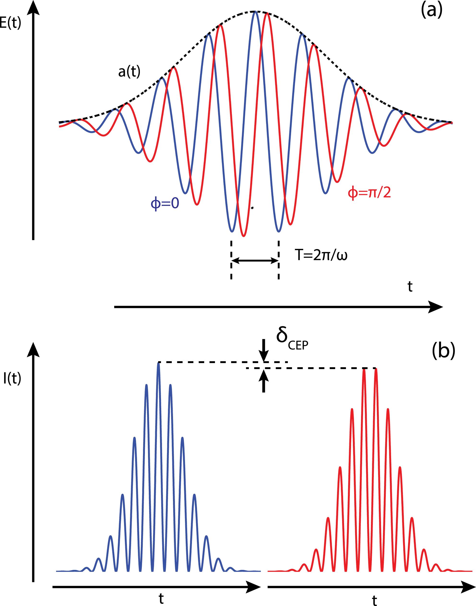
Few-cycle laser pulses are of interest due to the potential to easily access high peak intensities when tightly focused. Optical intensity is related to optical power via the simple relation $I=P/A$, where $P$ is the optical power and $A$ is the cross-sectional area. When discussing intensity in a pulsed laser system, it is important to be aware of the distinction between average power, $P_{av}$, and peak power, $P_{pk}$. Average power is the equivalent of measuring the laser power in a CW system, where the laser energy is integrated over a second to give the laser power. However, in a pulse laser system there are periods of zero laser power between pulses, which indicates that the power of each pulse must be higher than the averaged power measured. $P_{pk}$ is related to $P_{av}$ as follows $$\begin{eqnarray}P_{pk}=\frac{P_{av}}{\unicode[STIX]{x1D70F}_{p}f_{p}},\end{eqnarray}$$ (1) where $\unicode[STIX]{x1D70F}_{p}$ is the pulse duration and $f_{p}$ is the frequency of the pulse train. Therefore, $$\begin{eqnarray}I_{pk}=\frac{P_{av}}{\unicode[STIX]{x1D70F}_{p}f_{p}A}.\end{eqnarray}$$ (2) This relationship demonstrates that shortening the pulse duration can lead to high peak intensities. Current laser systems can reach pulse durations in the order of few femtoseconds, with pulse intensities up to the order of^[10–12]$10^{16}~\text{W}~\text{cm}^{-2}$, which are well suited for examining high-order nonlinear processes. The electric field of any laser pulse can be considered as a carrier wave inside an amplitude envelope function^[13], $$\begin{eqnarray}E(t)=a_{0}a(t)e^{-i(\unicode[STIX]{x1D714}t+\unicode[STIX]{x1D719})}+c.c.,\end{eqnarray}$$ (3) where $a_{0}$ is the peak amplitude of the envelope and $a(t)$ is a function that defines the shape of the envelope (such as Gaussian, $\text{sech}^{2}$, $\text{sin}^{4}$). $\unicode[STIX]{x1D719}$ determines the phase offset of the carrier wave from the envelope function and is known as the carrier-envelope phase (CEP). For pulses that contain many oscillations of the carrier wave the CEP has little relevance^[14]. However, for few-cycle pulses, the CEP is an extremely important parameter. This stems from the temporal evolution of the electric field waveform, as the shorter the pulse length the more the relative position of the carrier wave peaks within the envelope effects the peak electric field magnitude. By adjusting the CEP, the effective point of release of electrons during the ionization process can be controlled. In turn, this allows for the control of electrons in the oscillating laser field^[15]. Also, as the relationship between the electric field amplitude and the intensity of the laser light is $I(t)\propto E^{2}(t)$, it provides a method of fine control of the peak laser intensity. For a typical Gaussian intensity envelope function, the term $\unicode[STIX]{x1D6FF}_{CEP}$ is defined as the difference in intensity between a pulse with $\unicode[STIX]{x1D719}=\unicode[STIX]{x1D70B}/2$ (sine pulse) and a pulse with $\unicode[STIX]{x1D719}=0$ (cosine pulse). The relationship between sine, cosine and $\unicode[STIX]{x1D6FF}_{CEP}$ is shown in Figure 1. The high peak intensities made available by few-cycle laser pulses create interactions with matter that are highly nonlinear. One form of nonlinearity of a material arises from perturbative interaction with an electric field. This is a function of its polarizability^[9]$P(t)$$$\begin{eqnarray}P(t)=\unicode[STIX]{x1D716}_{0}(\unicode[STIX]{x1D712}^{(1)}E(t)+\unicode[STIX]{x1D712}^{(2)}E^{2}(t)+\unicode[STIX]{x1D712}^{(3)}E^{3}(t)+\cdots \,),\end{eqnarray}$$ (4) where the order of $\unicode[STIX]{x1D712}$ represents the $n$th order of optical susceptibility in the material. For instance, $\unicode[STIX]{x1D712}^{(1)}$ represents linear optical processes while higher orders represent the nonlinear processes^[9]. Essentially, Equation (4) represents the interaction between the electric field amplitude of the light passing through the material and the electric dipoles in a material, whether they are permanent or induced. This in turn has effects on the propagation of the light. Each order of $\unicode[STIX]{x1D712}$ above the first order introduces different nonlinear effects, but the key concept here is that the nonlinear processes become more pronounced under higher electric field intensities, which is why few-cycle pulses are of interest to studies of nonlinear optics.

Of particular interest to generating few-cycle laser pulses is the nonlinear Kerr effect, which alters the effective refractive index experienced by the incident light. This effect arises from $\unicode[STIX]{x1D712}^{(3)}$ and can be represented as^[16]$$\begin{eqnarray}n(I)=n_{0}+n_{2}I,\end{eqnarray}$$ (5) where $n_{0}$ is the linear refractive index of the material and $n_{2}$ the nonlinear refractive index of the material. As travelling light typically does not have a uniform radial intensity distribution, at the high intensities required to manifest the nonlinear Kerr effect the effective refractive index for the light is higher at the centre of the beam than at the radially outer regions. This generates a self-lensing effect, which is focusing if $n_{2}>0$. In addition, the temporal evolution of the wave is affected by alterations to the phase velocity, which can temporally broaden the spectral profile of the pulse^[17]. Both of these effects can be utilized to provide control to the spectral profile of laser pulses of sufficient intensity.

It is possible to generate few-cycle laser pulses by utilizing the mode locking of a specifically designed cavity. Mode locking is an interference phenomena whereupon a large number of coherent longitudinal laser modes oscillate simultaneously in a laser cavity^[8]. If the modes are correctly phase locked they interfere with each other, resulting in an output that is typically zero except for a short pulse of intensity where constructive interference of the modes occurs. In frequency space, the distance between adjacent frequency modes is the inverse of the cavity round trip time $T_{p}$. This is intuitive, as the frequency of any standing wave in a cavity must be a multiple of^[18]$1/T_{p}$. It follows that the nonzero intensity pattern must repeat with a period of $T_{p}$ within the cavity, and if the cavity light is coupled into free space, the pulses of constructive interference of laser intensity must occur with a frequency of^[8]$1/T_{p}$.

The actual pulse length, $\unicode[STIX]{x1D70F}_{p}$ is related to the both $T_{p}$ and the number of longitudinal modes in the cavity ($N$). The more modes in the cavity, the stricter the conditions are for constructive interference, thus shortening the pulse length. In contrast, the more frequent the output pulses, the shorter the cavity must be and thus conditions for constructive interference are less restrictive^[18]. The pulse length can be approximated by^[19]$$\begin{eqnarray}\unicode[STIX]{x1D70F}_{p}\approx \frac{T_{p}}{N}.\end{eqnarray}$$ (6) In a similar manner, the peak pulse power can be approximated as $$\begin{eqnarray}P_{peak}\approx NP_{avg},\end{eqnarray}$$ (7) where $P_{avg}$ is the average power of the cavity output. This indicates that in order to achieve maximum intensity, and thus minimum pulse duration from a mode-locked laser for the purpose of this work, the number of longitudinal modes must be maximized.

The interaction of strong-field laser fields with matter is a topical field^[20–26]. Effects such as high harmonic generation (HHG), above threshold ionization (ATI) and nonsequential double ionization (NSDI) all arise from the ionization of gas atoms or molecules by strong-field, few-cycle laser pulses^{[8, 27]}. HHG, in particular, is an area of research with an immediate practical use, the generation of coherent XUV pulses^[22]. These phenomena have been described by a semiclassical theory called the ‘three-step model’ diagrammatically represented in Figure 2^[28]. The first step of the model is the tunnelling ionization of the electron by the strong-field laser pulse. The tunnelling process occurs as the high electric field strength near the peak of the pulse suppresses the Coulomb potential binding the electron to the nuclear core of the atom. If the potential is suppressed to a sufficient degree, the probability of an electron tunnelling through the potential barrier becomes likely. If the potential is suppressed even further the electron may even be ionized over the potential. The second step of the model is the driving of the free electron by the oscillating laser field. The final step of the model is the potential recollision of the electron with the parent atom depending on the trajectory imparted to the electron by the laser field.

In order to better understand the nonlinear effects arising from the three-step model, it is important to fully understand each step of the model. This review will cover the initial ionization. There are three broad regimes for ionization, each of which is defined by its physical method of ionization. The three ionization regimes, in order of intensity required to reach them are multiphoton ionization, tunnelling ionization and over-the-barrier ionization (OBI). In order to provide an estimation of where the regimes change, two important parameters will be introduced. The Keldysh parameter, $\unicode[STIX]{x1D6FE}$, is the standard method to determine whether multiphoton or tunnelling ionization is the dominant ionization method^[8]. $$\begin{eqnarray}\unicode[STIX]{x1D6FE}=\sqrt{\frac{I_{p}}{2U_{p}}},\end{eqnarray}$$ (8) where $I_{p}$ is the ionization potential of the medium, and $U_{p}$ is the kinetic energy imparted to an ionized electron by a linearly polarized oscillating electric field, known as the ponderomotive energy. The multiphoton regime is defined as $\unicode[STIX]{x1D6FE}>1$, and the tunnelling regime is defined in the region where^[8]$\unicode[STIX]{x1D6FE}<1$. $$\begin{eqnarray}U_{p}=\frac{Ie^{2}}{2c\unicode[STIX]{x1D716}_{0}m_{e}\unicode[STIX]{x1D714}_{0}^{2}},\end{eqnarray}$$ (9) where $I$ is the laser field intensity, $e$ is the charge of an electron, $c$ is the speed of light in vacuum, $\unicode[STIX]{x1D716}_{0}$ is the vacuum permittivity, $m_{e}$ is the mass of an electron and $\unicode[STIX]{x1D714}_{0}$ is the central frequency of the pulse. The Keldysh parameter arises from Keldysh’s work to find common theoretical ground between perturbative multiphoton ionization and tunnel ionization. Physically, the Keldysh parameter is an adiabatic ratio that compares the time required to ionize an atom in a strong field to the oscillation period of the ionizing radiation. When the period is long compared to the ionization time, the ionization process can be reduced to a problem with a static DC field component, from which tunnel ionization arises^[29]. The work of Keldysh utilized the strong-field approximation (SFA) to define a general analytic formula for atomic ionization. The SFA assumes that the laser field will not change the initial bound state of the atom and that an electron ionized into the continuum state does not feel the Coulomb force from the parent atom^[30]. $\unicode[STIX]{x1D6FE}$ was singled out as a parameter that could be examined at two extremes. For the case where $\unicode[STIX]{x1D6FE}>1$, the optical frequency is high and the intensity low. The high frequency prevents the electron from tunnelling through the potential barrier in the period during the oscillation cycle where the electric field is high enough to allow tunnelling, which is the reason why multiphoton ionization is dominant in this regime. Likewise, for the opposite extreme where $\unicode[STIX]{x1D6FE}<1$, the optical frequency is low and the intensity is high, where there is ample time for the electron to tunnel through the potential barrier in each cycle. This essentially makes the Keldysh parameter a measure of how quickly the electric field of the laser oscillates compared to the time it takes for an electron to tunnel through the Coulomb barrier.

A general examination of tunnelling ionization in a strong electric field was carried out by Ammosov, Delone and Krainov in 1986^[31], and the result is known as ADK theory. The theory provides an analytical equation that would give the probability of an electron tunnelling out of the parent atom’s potential well under the influence of a high amplitude alternating electric field.

The work of Ammosov et al. builds on work performed by Perelomov et al.^[32], where the probability for ionization of atomic hydrogen is given by $$\begin{eqnarray}\displaystyle w & = & \displaystyle C_{n^{\ast }l^{\ast }}^{2}\sqrt{\frac{3F}{\unicode[STIX]{x1D70B}F_{0}}}E_{0}\frac{(2l+1)(l+|m|)!}{2^{|m|(|m|)!(l-|m|)!}}\ldots \nonumber\\ \displaystyle & & \displaystyle \times \,\left(\frac{2F_{0}}{F}\right)^{2n^{\ast }-|m|-1}\exp \left(-\frac{2F_{0}}{3F}\right),\end{eqnarray}$$ (10) where $E_{0}$ is the energy of the atomic state, $l$ and $m$ are the orbital and magnetic quantum numbers of the atom, $F$ is the electric field amplitude, $F_{0}=(2E_{0})^{3/2}$, $n^{\ast }$ is the effective principle quantum number given by $n^{\ast }=Z(2E)^{-1/2}$ and $Z$ is the charge of the ionic core. The terms of this equation arise from three different considerations. The $3F/\unicode[STIX]{x1D70B}F_{0}$ term results from averaging over the period of the field, the $2F_{0}/F$ term arises from the Coulomb interaction^[33] and the remainder is the result of the probability of tunnelling through a short range potential. Equation (10) arises by considering the evolution of an electron wavefunction tunnelling through the atomic potential into a Volkov wavefunction. The evolution is influenced by the electric field of the incident laser field and its quasi-classical perturbation of the atomic potential. In this equation, $C_{n^{\ast }l^{\ast }}^{2}$ is a dimensionless constant that is only known for the hydrogen atom. The work of Ammosov et al. was to find an approximation for $C_{n^{\ast }l^{\ast }}^{2}$ that could be applied to any target atom.

Consider the electron wavefunction, $\unicode[STIX]{x1D6F9}$, in the region where the field from the atomic potential is weak, but the effect of the external laser field can be neglected^[31]$$\begin{eqnarray}\displaystyle \unicode[STIX]{x1D6F9}_{n^{\ast }lm}(r) & = & \displaystyle C_{n^{\ast }l^{\ast }}\left(\frac{Z}{n^{\ast }}\right)^{1/2}\left(\frac{Z}{n^{\ast }}\right)^{n^{\ast }-1}\ldots \nonumber\\ \displaystyle & & \displaystyle \times \,\exp \left(-\frac{Zr}{n^{\ast }}\right)Y_{lm}\left(\frac{\boldsymbol{r}}{r}\right).\end{eqnarray}$$ (11) The effective principal quantum number $n^{\ast }$ is defined as $n^{\ast }=n-\unicode[STIX]{x1D6FF}_{l}$, where $\unicode[STIX]{x1D6FF}_{l}=n-(2E)^{-1/2}$ is the quantum defect. This allows the effective orbital quantum number to be defined as $l^{\ast }=l-\unicode[STIX]{x1D6FF}_{l}\equiv n_{0}^{\ast }-1$. Now consider the asymptotic form of a radial wavefunction of an arbitrary electron in a Coulomb potential^[34]$$\begin{eqnarray}R_{nl}=\frac{2^{n}Z^{1/2}(Zr)^{n-1}}{n^{n+1}((n+l)!(n-l-1)!)^{1/2}}\exp \left(-\frac{Zr}{n}\right).\end{eqnarray}$$ (12) By equating the coefficients between Equations (11) and (12) and replacing the quantum numbers $n$ and $l$ with their effective versions $n^{\ast }$ and $l^{\ast }$ it is possible to find an analytical form for $C_{n^{\ast }l^{\ast }}^{2}$ for an arbitrary atom of any atomic state. This is a valid comparison as the conditions for the wavefunction in Equation (11) still imply influence from the ionic core potential. After application of the asymptotic Stirling factorial formula^[35], this gives $$\begin{eqnarray}|C_{n^{\ast }l^{\ast }}|^{2}=\frac{1}{2\unicode[STIX]{x1D70B}n^{\ast }}\left(\frac{4e^{2}}{n^{\ast 2}-l^{\ast 2}}\right)^{n^{\ast }}\left(\frac{n^{\ast }-l^{\ast }}{n^{\ast }+l^{\ast }}\right)^{l^{\ast }+1/2},\end{eqnarray}$$ (13) where $e=2.718\ldots \,$. The result for Equation (13) can be substituted into Equation (10) to provide a probability of tunnelling ionization for an arbitrary atom in an arbitrary electric field, $$\begin{eqnarray}\displaystyle w & = & \displaystyle \left(\frac{3}{2\unicode[STIX]{x1D70B}}\right)^{3/2}\frac{Z^{2}}{3n^{\ast 3}}f(l,m)\left(\frac{4e^{2}}{n^{\ast 2}-l^{\ast 2}}\right)^{n^{\ast }}\ldots \nonumber\\ \displaystyle & & \displaystyle \times \,\left(\frac{n^{\ast }-l^{\ast }}{n^{\ast }+l^{\ast }}\right)^{l^{\ast }+1/2}\left(\frac{2Z^{3}}{n^{\ast 3}F}\right)^{2n^{\ast }-|m|-3/2}\ldots \nonumber\\ \displaystyle & & \displaystyle \times \,\exp \left[\frac{-2Z^{3}}{3n^{\ast 2}F}\right],\end{eqnarray}$$ (14)$$\begin{eqnarray}\displaystyle f(l,m) & = & \displaystyle \frac{(2l+1)(l+|m|)!}{2^{|m|}(|m|)!(1-|m|)!}.\end{eqnarray}$$ (15) Equation (14) was the result of Ammosov, Delone and Krainov’s work and is known as ADK theory. However, ADK theory, while making some insightful assumptions to approximate a solution, suffers in accuracy for two reasons. Firstly, it utilizes quasi-classical perturbation theory in the process of generating the expression for ionization rate, making it less accurate than a fully complete quantum mechanical model. Secondly, due to the assumption that the electron wavepacket is not affected by the Coulomb potential of the atomic core during the ionization process, the theory does not deal with OBI well, where for extremely high laser field intensities, the electric field suppresses the barrier to the point where the valence electron can be promoted directly to the continuum^[22]. The difference between the tunnelling ionization and OBI processes are highlighted in Figure 3.

OBI arises from the classical consideration of the interaction between a high electric field and the atomic Coulomb potential that binds the valence electron to the atom^[36]. For linearly polarized laser radiation it occurs in the regime where $$\begin{eqnarray}E_{bs}\geqslant \frac{I_{p}^{2}}{4Z}.\end{eqnarray}$$ (16) Typically Equation (16) is determined in atomic units (a.u), for which the equivalence to units more common in the literature are given as follows: electric field strength, $E$, $1~\text{a.u.}\equiv 5.14\times 10^{9}~\text{V}~\text{cm}^{-1}$; atomic core charge of the ion, $Z$, $1~\text{a.u.}\equiv 1.602\times 10^{-19}~\text{C}$; the ionization potential of the atom, $I_{p}$, $1~\text{a.u.}\equiv 27.21~\text{eV}$.

As the relationship between the intensity of a laser beam and electric field is given by $I~[\text{W}~\text{cm}^{-2}]=|E~[\text{V}~\text{cm}^{-1}]|^{2}/(2Z_{0})$ where $Z_{0}=377~\unicode[STIX]{x03A9}$ is the impedance of free space, it is possible to determine the field intensity where OBI becomes dominant, $I_{bs}$.

ADK theory does not provide a complete description of ionization with a high intensity laser field in general, in particular where the intensity regime is high enough that OBI is a significant contributing process. This has been recognized, and several attempts have been made to overcome this. Initially attempts to model this type of ionization was based on modifying ADK theory to account for barrier suppression ionization. One modification in particular was provided by Krainov and Shokri^{[22, 37, 38]}. In this work, a Coulomb correction is introduced to the Volkov wavefunction. This correction assumes a stronger interaction between the ionic core and the released electron, which alters the Volkov wavefunction when solving as per the ADK method. For low laser intensities, the solution reduces to the ADK theory solution of ionization probability^[38]. Under the Coulomb correction, the probability for ionization is given by^[22]$$\begin{eqnarray}\displaystyle w(t) & = & \displaystyle \unicode[STIX]{x1D714}_{p}|C_{n\ast }|^{2}\left(\frac{4\unicode[STIX]{x1D714}_{p}}{\unicode[STIX]{x1D714}_{t}}\right)^{2n\ast -1}\exp \left(-\frac{4\unicode[STIX]{x1D714}_{p}}{3\unicode[STIX]{x1D714}_{t}}\right),\end{eqnarray}$$ (17)$$\begin{eqnarray}\displaystyle \unicode[STIX]{x1D714}_{p} & = & \displaystyle \frac{I_{p}}{\hbar },\end{eqnarray}$$ (18)$$\begin{eqnarray}\displaystyle \unicode[STIX]{x1D714}_{t} & = & \displaystyle \frac{eE(t)}{(2mI_{p})^{1/2}}.\end{eqnarray}$$ (19)

Another attempt to modify ADK theory to account for OBI was performed by Tong and Lin^[39]. In this work, the authors propose a modified form of the ADK equation to give the total ionization probability, $$\begin{eqnarray}w(E)=w_{ADK}\exp \left(-\unicode[STIX]{x1D6FC}\frac{Z^{2}E}{4I_{p}^{5/2}}\right).\end{eqnarray}$$ (20) The exponential correction term is expressed in terms of the scaled field strength and ionization potential, and is dependent upon the empirical value $\unicode[STIX]{x1D6FC}$. Values for $\unicode[STIX]{x1D6FC}$ for different atomic species can be found in Ref. [39].

The main advantage of using ADK theory-based methods for calculating ionization probability is that they are computationally inexpensive. With the recent increase in availability of computer processing time however, it is becoming increasingly popular to numerically solve the time-dependent Schrödinger equation for the electron, with the results dependent upon the approximations and methods used^[40]. These methods are varied, but a sample would include work done using the S-matrix method with the SFA^{[41, 42]}, work done by propagating the time-dependent wavefunction in the integral form^[40] and work done with a matrix iterative approach^[43].

Following the introduction of the Keldysh parameter as a metric for determining strong-field regime, there was almost two decades where examination of strong-field ionization of atoms could not be performed experimentally due to the lack of lasers capable of providing the electric field amplitude required to reach the strong-field regime. The earliest examples of work examining the strong-field ionization of atoms was performed in the early 1980s at the Australian National University with 1064-nm Nd:glass lasers capable of 1.8 J per 25 ps pulse^{[44, 45]}. These works examined the ionization of helium and argon, comparing the expected electron energies of perturbative multiphoton ionization and a rough comparison of Keldysh tunnelling theory to their observed results for different ionization states. At this point in time, ADK theory had not been developed, but the results strongly disagreed with the expected perturbative electron energies and there was observation of the effect of the ponderomotive force on an ionized electron^[44].

Other attempts to observe strong-field regime ionization before the development of ADK theory were performed by Chin et al. and focused on utilizing a lower-frequency laser source^[46–48]. These experiments were performed with the 10.55 and $9.55~\unicode[STIX]{x03BC}\text{m}$ lines of a $\text{CO}_{2}$ laser capable of producing multijoule 1.1-ns pulses, using atomic noble gas targets. The reasoning behind this approach was that with the lower frequency there would be less photon energy, reducing the contribution of multiphoton ionization. This was observed in the results, where focal volume averaged ion yields were fitted to multiphoton theory and Keldysh theory. The disagreement with a multiphoton approach convinced the authors that tunnelling ionization was observed.

Shortly after the appearance of ADK theory, the first example of OBI was observed by Augst et al.^{[49, 50]} in 1989. This work reverted back to shorter pulses, utilizing a Nd:glass laser system capable of producing 100-mJ, 1-ps pulses at a wavelength of 1053 nm to ionize noble gas atoms. Observation of the ion yield results compared favourably to the expected ADK results, but also compared favourably to a simple classical model involving the superposition of an atomic Coulomb potential with a static electric field^[36]. This led the authors to the conclusion that the electric field of the laser pulse was reaching intensities such that OBI could occur. This sparked interest in the development of an ADK solution which dealt with the occurrence of OBI as noted in Section 1.3.

Around the same period of time it was noted that the interaction of linearly polarized strong-field pulses with atoms was generating HHG. The first observation of HHG was reported by McPherson et al.^[51] in 1987, utilizing Xe as the gas target. At the time, the authors were unsure as to the exact mechanism, but believed it to be a multiphoton process in nature and were capable of observing the 17th harmonic. Further investigation correlated high-order harmonics to ATI electron peaks^{[52, 53]}, establishing the connection between tunnelling ionization and HHG. Studies of HHG were continued^{[54, 55]}, but it was not until the development of Corkum’s three-step model^[28] that the mechanism for HHG was fully understood. Other experiments in strong-field ionization during the mid to late 1990s concentrated on expanding the understanding of HHG^{[56, 57]} in order to achieve a tabletop source of coherent attosecond pulses.

Around the turn of the millennium, reaction microscopes began making their way into the field of strong-field laser/matter interaction as detectors, allowing experimentalists to measure the momentum of the ionization products^[58]. The development of such devices is reviewed in Section 1.5. The new measurement options generated renewed interest in strong-field ionization as a path to improving understanding of atomic electron structure and dynamics. For instance, studies in multiple ionization of noble gas atoms^{[23, 59, 60]} utilized discrepancies in expected electron momentum to identify that not all higher-order ionizations were a result of tunnel ionization through sequential optical cycles. These works identified that the returning electron could cause secondary ionization via recollision (NSDI), or excite the atom to a higher energy level, changing the ionization potential of the target for the following optical cycle. The effects of atomic structure on the dominant multiple ionization process were also examined by comparing electron momentum distributions of Ne, Ar and He atoms^[61]. This particular experiment lacked examination of different atomic states of a single atomic species, possibly allowing nuclear spin and inner electron core dynamics to affect the results.

During the same time period, the rising availability and use of few-cycle strong-field laser pulses generated interest in the effects of few-cycle pulse properties on the ionization process. Initial experiments indicated that there was a shot-by-shot asymmetry in electron yields^[24], which was attributed to the random phase difference between the carrier wave and the envelope function of the laser pulse, also known as the CEP. The CEP affects few-cycle pulses to a greater extent than longer pulses as changes in the CEP greatly alters the peak electric field of a few-cycle pulse (see Section 1.2 for details). Several experiments were performed in order to specifically measure these effects^{[60, 62]} or use CEP to control the ionization dynamics^{[15, 21, 63]}. The ultimate application of this line of research was the CEP single-shot phase meter, a device that utilizes asymmetry in a calibrated ATI spectrum to determine the CEP phase of a single laser pulse^[64].

Given the broad depth of detection devices and fine control over CEP now available, experimentation has recently branched into several diverse fields. These include the examination of ATI spectra of atomic targets with elliptically polarized light^{[65, 66]}, using CEP to time the release of electrons during sequential ionization^[67], or utilizing the ionized electron energy measurements from atomic hydrogen to provide an accurate calibration of laser intensity^[10].

Time-of-flight (TOF) mass spectrometers have been a workhorse for the detection of charged particles for more than 60 years^[68]. TOF spectroscopy involves accelerating charged particles through a known electric field over a known distance onto a detector. Consider an ideal case of charge particle initially accelerated by an electric field. In this case, the potential energy of the charged particle in the electric field, $E_{p}$, is converted to kinetic energy, $E_{k}$, as follows $$\begin{eqnarray}\begin{array}{@{}rcl@{}}\displaystyle E_{p}\ & =\ & qV,\\ \displaystyle E_{k}\ & =\ & {\textstyle \frac{1}{2}}mv^{2},\\ \displaystyle E_{p}\ & \equiv \ & E_{k},\\ \displaystyle qV\ & =\ & {\textstyle \frac{1}{2}}mv^{2},\end{array}\end{eqnarray}$$ (21) where $q$ is the charge of the particle, $V$ is the potential of the accelerating electric field, $m$ is the mass of the particle and $v$ is the velocity of the particle. The charged particle is then passed into a field-free TOF tube, where it proceeds a known distance towards the detection device. Simple application of the equations of motion under constant acceleration and the result from Equation (21) shows that the time taken for the charged particle to travel up the tube and reach the detector is given by $$\begin{eqnarray}t=\frac{s}{\sqrt{2V}}\sqrt{\frac{m}{q}},\end{eqnarray}$$ (22) where $s$ is the length of the TOF tube. In a real world scenario it is exceedingly difficult to design a TOF such that external fields do not infringe in the TOF tube at some point, and as a result we let $(s/\sqrt{2V})\rightarrow \unicode[STIX]{x1D70C}$, where $\unicode[STIX]{x1D70C}$ is a constant that relates to the settings and characterization of the actual experimental setup. Equation (22) indicates that the time taken for the particle to reach the detector is proportional to its charge-to-mass ratio, $q/m$, thus the use of TOF as a mass spectroscopy technique.

TOF detectors are typically a simple anode^[68]. However, in situations where the expected charged particle count is low, a signal multiplier may be required^[69]. The microchannel plate (MCP) is a common signal multiplier that was first developed in 1961 at Bendix Research Laboratories^[70]. The MCP is a device that situates an array of single straight channel electron multipliers parallel to each other on a substrate^[69]. Each straight channel electron multiplier is a device that generates a cascading secondary emission electron response from an initial charged particle, and the gain of each straight channel electron multiplier is given by^[71]$$\begin{eqnarray}G=\unicode[STIX]{x1D6FE}_{0}\unicode[STIX]{x1D6FE}^{l/d},\end{eqnarray}$$ (23) where $\unicode[STIX]{x1D6FE}_{0}$ is the initial secondary electron yield from the collision of the ion with the channel, $\unicode[STIX]{x1D6FE}$ is the mean secondary electron yield when an avalanche electron strikes the channel wall, $l$ is the length of the channel and $d$ is the diameter of the channel. Gain scalability is therefore limited by the ability of the manufacturing process to make thinner channels. Arrays of the straight single channel electron multipliers therefore generate electron bunches, which can be picked up by a detection device that would not normally be sensitive to a single charged particle, such as an electrode attached to an ammeter^[71]. A schematic diagram of an MCP is given in Figure 4.

There have been many improvements to MCP’s since their first demonstration. Improvement of the geometry of the channels reduced the effects of space charge effects near the output of the channels to increase gain^{[72, 73]}. Introduction of the chevron dual-layer MCP design in the early 1970s reduced ion feedback (whereby positive ions are generated at the output, which induces a secondary electron bunch) and increased the total gain of the system^{[69, 74]}. The z-stack tri-layer MCP design was examined in the early 1980s, which saw a further improvement in gain^[75]. Current examples of MCPs typically achieve gains of^{[76, 77]}${\approx}10^{7}$.

The next step in the evolution of detector was the marriage of position sensitive detectors (PSDs) to the TOF apparatus. This would not only allow information about the $m/q$ ratio from TOF measurements, but would allow the momentum of detected particles from the ionization products to be determined. The earliest examples of PSDs arose from standard anode technology in the late 1970s^{[78, 79]}. These devices utilized multiple anodes separated by insulators. The anodes pick up the electron bunch as a current signal, but as the electron bunch output by the MCP has a distribution, each anode will detect a different current. By using comparator circuitry, the location of the centre of the electron distribution could be determined and therefore the location of the initial particle strike could be determined. These devices were capable of resolving down to $100~\unicode[STIX]{x03BC}\text{m}$ with a dead time of^[78]${\approx}1~\unicode[STIX]{x03BC}\text{s}$.

Improvement in PSD resolution came with the development of the delay-line detector in the late 1980s^{[80, 81]}. A one-dimensional delay-line detector consists of a pair of conducting wires wrapped in an alternating fashion around an insulating material that covers a central electrode core. The alternating pairs of wires are connected to differential amplifiers (one at each end of the wire pair), and a DC voltage is applied across the wires such that all incident charge is collected on one wire. Incident electron bunches are detected at both differential amplifiers. By comparing the timing of the arrival of the signal at both differential amplifiers, the location where the electron bunch struck the wire pair can be determined. 2D delay-line detectors incorporate a second pair of wire detectors at right angles to the first, with the voltage across the lines balanced so as to the electron bunch is evenly distributed collected by both pairs of wires. Initial results with this detector provided resolutions of $25~\unicode[STIX]{x03BC}\text{m}$ with a dead time of^[81]${<}1~\unicode[STIX]{x03BC}\text{s}$. More recent improvements include general speed advances in timing circuitry and the development of the Hexanode style delay-line detector, which reduces dead times down to 5 ns^[82].

The application of these advances in detection technology to the field of ionization by energetic impact led to the creation of the first cold target recoil ion momentum spectroscope (COLTRIMS) devices in the mid 1990’s^{[58, 83]}. The first COLTRIMS was designed to be an improvement in the detection of low-energy electrons from atom–heavy ion collisions^[58], in which a supersonic jet of He cooled to 10 mK collided with a heavy ion beam in an interaction region. $\text{He}^{+}$ ions were extracted from the interaction region with an applied electric field and passed through a TOF region onto an MCP wedge and strip anode PSD. Electrons were extracted in the opposite direction into a similar TOF device. This experimental setup gave the longitudinal and transverse momentums of the ions and electrons which could be correlated to provide coincidence measurements, with the background signal reduced to the order of^[58]$10^{-4}$.

COLTRIMS improvement up until the present has been largely driven by attempts to reduce the dead time of the device, and therefore increase the amount of collected data^[84]. This is because improvements in momentum resolution are dependent upon the extraction voltage, not issues with application of the technology. A higher voltage gives a lower comparative transverse final velocity of the charged product after leaving the extraction E-field. However, if the extraction voltage is too low, charged products may not be captured by the TOF, making momentum resolution an experimental trade-off with detection efficiency. Typical momentum resolutions for ions range between 0.1 and 0.35 atomic units depending on experimental conditions^[85–87]. Reductions in dead time by incorporating delay-line detectors increased the data taking frequency to MHz^[88]. Introducing delay-line detectors also reduced the dead time between multiple hits to 10 ns, increasing the capability of the COLTRIMS to detect multiple ionization events per interaction^{[88, 89]}.

Noble gas atoms have a ground-state configuration with a full outer $np$ shell. The first excited state of such atom has an $(n+1)s$ electron that is free to couple with the electron hole in the otherwise full $np$ orbital. This gives four separate degrees of angular momenta to couple, the spin and orbital angular momentum of the valence electron and the spin and orbital angular momentum of the electron core. In order to complete this coupling, the $j\ell$ coupling scheme is typically used^[90]. In this coupling scheme, the inner electron core is assumed to be well LS coupled and completes coupling first. This gives a total angular momentum of the electron core, $j_{c}$. The core angular momentum then couples to the orbital angular momentum of the valence electron such that $K=j_{c}+\ell _{e}$. The coupling is completed when $K$ couples with the spin of the valence electron such that $J=K+s_{e}$. $j\ell$ coupling notation is denoted by $$\begin{eqnarray}(\,^{2S_{c}^{\prime }+1}L_{J_{c}^{\prime }}^{\prime })n_{e}\ell _{e}[K]_{J},\end{eqnarray}$$(24) where the term in the brackets is the LS coupling term for the electron core and $n_{e}$ is the principle quantum number of the valence electron.

Treatment of electron–hole coupling is similar to electron–electron coupling, and this treatment will begin with that. This gives an effective coupling structure of $np^{1}(n+1)s^{1}$. By examining the potential quantum numbers of this coupling, four LS coupling states are generated from the electron core, a singlet and a triplet state. As electron–hole coupling is in effect, the energy levels of the triplet state are inverted compared to electron–electron coupling^[91]. To take an example, in the case of neon this coupling manifests as the highest energy state in the manifold being $^{1}P_{1}$ singlet followed by an inverted $^{3}P_{J}$ triplet^[91]. The LS coupled core undergoes the $j\ell$ coupling, and the resultant $j\ell$ first excited states can by written as linear mixtures of the core LS coupled states as follows^[92], $$\begin{eqnarray}\displaystyle \,^{2}P_{3/2}3s[3/2]_{2} & = & \displaystyle 3^{3}P_{2},\end{eqnarray}$$(25)$$\begin{eqnarray}\displaystyle \,^{2}P_{3/2}3s[3/2]_{1} & = & \displaystyle \unicode[STIX]{x1D6FD}3^{1}P_{1}+\unicode[STIX]{x1D6FC}3^{3}P_{1},\end{eqnarray}$$(26)$$\begin{eqnarray}\displaystyle \,^{2}P_{1/2}3s[1/2]_{0} & = & \displaystyle 3^{3}P_{0},\end{eqnarray}$$(27)$$\begin{eqnarray}\displaystyle \,^{2}P_{1/2}3s[1/2]_{1} & = & \displaystyle \unicode[STIX]{x1D6FC}3^{1}P_{1}+\unicode[STIX]{x1D6FD}3^{3}P_{1},\end{eqnarray}$$(28) where $\unicode[STIX]{x1D6FC}^{2}+\unicode[STIX]{x1D6FD}^{2}=1$. There are two states that are strongly LS coupled and can thus be represented with the LS coupling scheme, the $3^{3}P_{0}$ and the $3^{3}P_{2}$ states. Due to selection rules for optical transitions, these states can be neither optically excited nor can they decay via spontaneous emission, making them metastable. In order to reach these states, a different excitation method is required, typically collisional. As this work considers well LS coupled states, LS coupling nomenclature will be used. Figure 5 gives the energy level ensemble of neon as an example.

Huismans et al. presented a study done with metastable xenon atoms as the target for tunnel ionization in order to examine holography using photoelectrons from the ionization process^[93]. This was performed in order to attempt to examine the electron dynamics of an ionizing system, with the aim to extract temporal and phase information for the ionized electron from the data.

The basis of holographic electron imaging is displayed in Figure 6. The process requires observing an interference pattern between a reference wave, which is emitted from the source and does not interact with the atomic target, and a signal wave, which scatters off the target, storing information about its structure. The phase difference between the electron waves is given by $\unicode[STIX]{x1D6E5}\unicode[STIX]{x1D711}=(k-k_{z})z_{0}$ where $k$ is the total momentum, $k_{z}$ is the momentum in the $z$ direction and $z_{0}$ is the displacement from the scattering centre^[93].

In order to observe the interference, it is necessary to eliminate as much interference from the atomic core as possible. This was the reason for the use of tunnel ionization in Huismans et al.’s work; the active electron is released some distance through the Coulomb barrier away from the ionic core. In addition, the authors note that in order to obtain acceptable results using their holographic imaging methods, two conditions needed to be fulfilled. The first is that the oscillation of the electron needed to be large ($\unicode[STIX]{x1D6FC}\gg 1$ Å), and the second is that the ponderomotive energy of the electron is large ($U_{p}\gg \hbar \unicode[STIX]{x1D714}_{laser}$). Both these properties scale with $\unicode[STIX]{x1D706}_{laser}^{2}$ and $I$. The laser source utilized by the authors was a $7~\unicode[STIX]{x03BC}\text{m}$ wavelength mid-IR pulse from the FELICE beamline at the Free Electron Laser for Infrared Experiments (FELIX) facility^[94]. Metastable xenon was chosen as the target of choice as the low ionization potential ($I_{p}=3.8$ eV) combined with the wavelength of the laser source allowed ionization to occur within the tunnelling regime for the laser intensities used ($\unicode[STIX]{x1D6FE}=0.8{-}1.3$)^[93].

The experiment performed by Huismans et al. recorded the momentum distribution and angle-integrated photoelectron spectra across six laser intensities ranging from $1.9\times 10^{11}$ to $7\times 10^{11}~\text{W}~\text{cm}^{-2}$ using a velocity map imaging spectrometer (VMI) integrated with the FELICE laser cavity^[95]. The results are shown in Figure 7. A beautiful set of ‘side lobes’ resulting from holographic interference exists in the high intensity results that run parallel to the direction of laser polarization. These side lobes gradually become less visible and completely disappear at the intensities below $3.2\times 10^{11}~\text{W}~\text{cm}^{-2}$. This occurs when the ionization regime moves from the tunnelling regime to the multiphoton regime as defined by the Keldysh parameter $\unicode[STIX]{x1D6FE}$ changing from 0.8 to 1.5. The other major feature to be observed are the rings around zero momentum, which are caused by backscattered electrons in higher-order ATI^{[96, 97]} and not related to the electron interference^[93].

Huismans et al. confirm the observation of the holographic interference pattern by comparing the experimental results to both full TDSE calculations, and Coulomb-corrected strong-field approximation (CCSFA) calculations, as per Figure 8. This work was a wonderful experimental demonstration of recording holographic structures for exploring the electron and hole dynamics in the ionization process, and is a strong test case for the study of more complicated molecular systems, such as work performed in Ref. [98].

As discussed in Section 1.3, the application of a high intensity light pulse to an atom can cause ionization. Experiments for these interactions with noble gases have been performed and uncovered various phenomena such as NSDI with long and short pulse lengths^{[59, 99]} and HHG^[25]. Characterization experiments have also been performed, for example the effects of polarization of the ionizing beam on the ionization rate of helium and neon^[100] and the effects of atomic shell structure on NSDI^[61]. Investigation the strong-field ionization of metastable neon ($\text{Ne}^{\ast }$) was recently performed by Calvert et al.^[101]. This work was pursued for a number of reasons. Firstly, the low ionization potential of metastable neon (5.1 eV) allows for investigations of OBI effects using laser systems that are relatively common in the strong-field community. Secondly, comparisons between ground-state and metastable-state neon allow for the examination of ionization effects that are dependent upon the valence electron shell, without altering the nucleus and electronic core. In addition, the single-photon dipole allowed cooling transition of $\text{Ne}^{\ast }$ allows the spin polarization of the valence electron by pumping with correctly oriented circularly polarized light, allowing another method of examining the role of the initial atomic state on the ionization dynamics of the system.

In comparison to the work done on the ionization of metastable xenon targets by Huismans et al.^[93] using a $7~\unicode[STIX]{x03BC}\text{m}$ laser, the work done by Calvert et al. reaches higher peak laser intensities, allowing for an examination of both tunnelling ionization and OBI effects.

The main purpose of this particular experiment was to examine the strong-field ionization yield of $^{3}P_{2}$ neon ensembles that are spin polarized. However, as the initial strong-field ionization is an important process to understand, it was investigated first. To make any valid comparison between theory and experiment required the folding of experimental parameters with the theory. This required modelling that takes into account the size and shape of both the atomic beam and the laser pulse, as well as the temporal structure of each laser pulse.

In order to determine the total ion yield it was necessary to determine the ionization fraction at varying laser intensities. This was performed using Matlab by solving Equation (29), as per the method used by Gibson^[102]. $$\begin{eqnarray}\unicode[STIX]{x1D702}(t)=1-\exp \left[-\int _{-\infty }^{t}dt^{\prime }w(t^{\prime })\right],\end{eqnarray}$$ (29) where $\unicode[STIX]{x1D702}(t)$ is the total ionization fraction caused by a laser pulse interacting with the atom after time $t$ and $w(t^{\prime })$ is the instantaneous ionization rate at time $t^{\prime }$. The $w(t^{\prime })$ term is entirely dependent on the theory used to determine ionization rate. In this work two theories were examined: ADK- and a TDSE-based theory provided by Tong.

ADK theory uses the ionization rate equation given in Equation (14). In order to calculate a solution for Equation (29), $t$ was set such that it encompassed the whole of a laser pulse. The range $0\rightarrow t$ was then broken up into small fractions such that $\unicode[STIX]{x1D6FF}t=t/10\,000$ so as to solve Equation (29) as a sum of elements. This division provided convergence to lower than 0.001%. The electric field of the laser was generated at all points $t^{\prime }=n\unicode[STIX]{x1D6FF}t$, where $n$ is the iteration number, as per $$\begin{eqnarray}E(t^{\prime })=E_{0}\cos (\unicode[STIX]{x1D714}_{0}t^{\prime })\exp \left[\frac{-(t^{\prime })^{2}}{\unicode[STIX]{x1D70F}_{pul}^{2}}\right],\end{eqnarray}$$ (30) where $E(t^{\prime })$ is the electric field amplitude at time $t^{\prime }$, $E_{0}$ is the peak amplitude of the electric field, $\unicode[STIX]{x1D714}_{0}$ is the central frequency of the laser pulse and $\unicode[STIX]{x1D70F}_{pul}$ is the FWHM of the laser pulse. $E_{0}$ is a varying parameter, and is determined from the laser intensity as $E_{0}=\sqrt{I_{pk}\times 2Z_{0}}$ where $Z_{0}=377~\unicode[STIX]{x03A9}$. According to Equation (14), it is necessary to know several variables for the atom in order to solve for $w$. These are the orbital angular quantum number $\ell$, its projection $m_{\ell }$, the effective total quantum number $n^{\ast }$, the effective orbital quantum number $\ell ^{\ast }$ and the charge of the ionic core $Z$. These are all known for $\text{Ne}^{\ast }$ and do not vary over the time $t$. Likewise, the laser properties can all be measured experimentally. The experimental values are used to solve Equation (14) at all given times $t^{\prime }$, the results of which are then used to numerically solve the integral in Equation (29), to give an ionization fraction for any given simulated laser intensity $I_{pk}$. An example of the evolution of this system is given in Figure 9, where the time evolution of the electric field of a laser pulse is shown in blue. The associated $\text{Ne}^{+}$ fraction derived from parent ground-state neon atoms at any given time during the pulse is shown in green. It can be observed that as the electric field increases, the ionization fraction increases until it reaches unity. Higher peak electric field amplitudes result in the system reaching the unity ionization fraction at an earlier time, while lower electric field amplitudes will see the ionization fraction reaching unity at a later time, if the system is capable of achieving complete ionization.

Determining the ionization fraction for the TDSE equation at a given intensity was performed differently to the ADK approaches. TDSE data was provided by Tong giving the ionization fraction at a range of laser intensities from $1.0\times 10^{12}$ to $1.2\times 10^{15}~\text{W}~\text{cm}^{-2}$. These data were used to generate an interpolating spline which allows the ionization rate to be determined at any arbitrary intensity within that range. The ionization probabilities of the Ne $3s$ electron were calculated by solving the TDSE under the single-active electron approximation with the second-order-split operator method in the energy representation^{[40, 103]}. The model potential^[104] is calculated by using the density functional theory with self-interaction correction^[105], from which the calculated atomic ionization potentials are in good agreement with the measured ones. The numerical convergence was cross checked by comparing the ionization probabilities obtained from the integration of the ATI spectra and survival probability of the $3s$ orbital into the bound states. The two results are in agreement within a few percent.

The results returned from the theoretical models in Section 4.1.1 all refer to a single atom being ionized by a single pulse at a point in space. The experimental apparatus used by Calvert et al. could not reproduce these conditions as the laser beam is finite in size and the atomic beam can have more than one atom in the interaction region. As such there are different probabilities of ionization across a volume defined by the overlap between the laser and atomic beam. This makes total ion yield calculations nontrivial, as it is not simply a matter of multiplying the ionization fraction by the number of pulses that are passing through the interaction region in the model. It is possible to design the experiment such that it reduces focal volume effects by reducing the size of the interaction region as observed by the detection devices. Traditionally this is performed through aperturing between the interaction region and the detector^[106], which removes particles with energy that do not give them a trajectory through the aperture. A downside of this approach is the loss of potential signal, reducing the signal to noise ratio. Aperturing may also not be an option due to experimental restrictions. The multipurpose nature of the COLTRIMS prevents the use of aperturing in the work performed by Calvert et al. In their case, the ionization probability over the entire interaction region must be determined by integrating the ionization rate over the focal volume. This was performed for this experiment, with the method described below.

To perform the focal volume averaging to calculate the total ionization it was necessary to model the conditions of the interaction region and determine the expected yield of ions under those conditions. The model assumes that the laser beam is Gaussian and focused to a spot in the centre of the cylindrical atomic beam, with no astigmatism. This was justified from the atomic beam preparation and beam width measurements. The atomic beam is prepared through two 1.5 mm apertures separated by a distance of approximately 300 mm. Beam width measurements are given in Figure 10. Figure 11 displays a schematic of the modelled system. Due to the cylindrical nature of the atomic beam, the coordinate system was defined in cylindrical polar coordinates, $(r,\unicode[STIX]{x1D703},z)$. The $z$-axis is defined in Figure 11 as being the direction of propagation of the atomic beam. As solving symmetrically in $\unicode[STIX]{x1D703}$ simplifies the calculations, the $r$-axis is described as existing along the $\unicode[STIX]{x1D703}=0$ angular coordinate, as shown in Figure 11.

It is possible to define the integral for the total ion yield in the focal volume as $$\begin{eqnarray}\unicode[STIX]{x1D6FC}_{tot}=\int \unicode[STIX]{x1D6FC}(r,\unicode[STIX]{x1D703},z)\,dr\,d\unicode[STIX]{x1D703}\,dz,\end{eqnarray}$$ (31) where $\unicode[STIX]{x1D6FC}_{tot}=$ is the total ion yield. Due to the cylindrical symmetry of the system around the origin, it is possible to bring out the integration under $\unicode[STIX]{x1D703}$ as a constant $2\unicode[STIX]{x1D70B}$, giving $$\begin{eqnarray}\unicode[STIX]{x1D6FC}_{tot}=2\unicode[STIX]{x1D70B}\int \unicode[STIX]{x1D6FC}(r,z)\,dr\,dz.\end{eqnarray}$$ (32)$\unicode[STIX]{x1D6FC}(r,z)$ can be determined from the calculated ion fraction $w(r,z)$ and the atomic number density $D(r,z)$ such that $$\begin{eqnarray}\unicode[STIX]{x1D6FC}_{tot}=2\unicode[STIX]{x1D70B}\int w(r,z)D(r,z)\,dr\,dz.\end{eqnarray}$$ (33) In order to solve this integral, a grid was set up along the $r{-}z$ plane. The maximum values for the axes are dependent upon the width of the atomic beam in the $z$ direction $z_{abeam}$, and the $1/\text{e}^{2}$ width of the laser beam in the $r$ direction. The grid points were generated on these axes by dividing the maximum widths of the $r$ and $z$ directions by a grid sizing variable. The grid sizing variable provides a trade-off in that the higher the value, the finer the grid points and hence higher the resolution of the ionization grid map, but at the cost of a corresponding increase in computation time. For the calculations performed, a grid sizing variable of 20 was used, as after multiple iterations of testing the grid sizing variable was shown to converge to below 0.5% while retaining reasonable computation time (${\sim}20$ min). Once the grid points were defined, the intensity profile of the laser pulse was mapped onto the grid. This allowed the laser intensity at any point on the grid to be determined using the equation$$\begin{eqnarray}I(r,z)=\frac{I_{0}}{1+(\frac{z}{R_{z}})^{2}}\exp \left(\frac{-r^{2}}{w_{0}[1+(\frac{z}{R_{z}})^{2}]}\right).\end{eqnarray}$$ (34) This requires the input of the Rayleigh range, $R_{z}$, the radius of the beam waist at the focus, $w_{0}$, and the peak intensity of the laser at the centre of the focus, $I_{pk}$. At each grid point the laser intensity was used to generate an ionization fraction. For the case of ADK theory, the laser intensity is used in conjunction with Equation (29) and the appropriate ionization rate equation to generate the ionization fraction. For the TDSE case, the laser intensity was used in conjunction with the spline of ionization rates to interpolate an ionization fraction. This generated a 2D ionization fraction map.

The data from the 2D ionization fraction map was interpolated using a Piecewise Cubic Hermite Interpolating Polynomial (pchip) Matlab function between the grid points in both directions. These functions were solved over a grid that has the same maximum dimensions but has had the grid point density increased by a factor of 100, which resulted in a much finer 2D ionization map, as shown in Figure 12. The density factor increase was chosen as a trade-off between convergence (${<}0.5\%$) and computation time. The interpolated map is accurate to within 5% of an ADK ionization yield map of the same resolution that has not been interpolated, while being 3 orders of magnitude faster to compute. The interpolation process increases the resolution around the edges of the volumes of the pulse without the loss of ionization fraction information. As shown in Figure 12, there is a very steep ionization fraction gradient at the edges, where a large part of the ionization fraction information is located. Increasing the grid resolution in this manner increased the accuracy of the raw ion yield results by $(27\pm 5)\%$.

The effects of the atomic beam must be introduced into the script in order to determine the modelled total ion yield. The estimated atom flux in the interaction region was determined from the estimated gas source flux $\unicode[STIX]{x1D711}$, and the subtended solid angle of the interaction region, $$\begin{eqnarray}\unicode[STIX]{x1D719}=4\unicode[STIX]{x1D70B}\text{sin}^{2}\left(\frac{z_{abeam}}{s_{source}}\right),\end{eqnarray}$$ (35) where $s_{source}$ is the distance from the source nozzle to the interaction region and $z_{abeam}$ is the estimated width of the atomic beam.

From this flux data, a $z$-dependent atomic density profile of the interaction region was generated along the grid points in the $r{-}z$ plane, giving $D(r,z)$. As the atomic beam is assumed to be cylindrical with a uniform density, this projects as a top-hat beam profile along the $r{-}z$ plane. With grid solutions for $D(r,z)$ and $w(r,z)$ the integration in Equation (33) could be completed by summation across all grid points in the $r{-}z$ plane. This gives the theoretical ion yield from a single laser pulse an example of which is shown in Figure 13. In order to complete the modelling, this single-shot yield was multiplied through by the total number of laser pulses, $n$.

Figure 14 outlines the differences in applying different theories to the same modelling parameters for $^{3}P_{2}$ neon. There are a few points to highlight here. The first one is that in the ADK data there is a region of laser intensity from 0 to $0.2~\text{W}~\text{cm}^{-2}$ where the ionization yield remains low due to the relatively low electric field strength. This does not appear in the full TDSE approximation, where multiphoton ionization and OBI is modelled (see Figure 15 for the fine structure transitions in neon). Secondly, there is almost no qualitative difference in the theoretical curves after the saturation points are reached. The differences in the theories are therefore best highlighted in the region before saturation, where it can be noted that the theories that consider OBI rise up to saturation region at lower intensities than ADK theory does, in turn indicating that the inclusion of OBI electrons increases the ion yield in this modelling. It is likely that this is a manifestation of volume effects at the edge of the laser beam as the intensity increases.

This work also examined the effect of pumping the $\text{Ne}^{\ast }$ atoms into stretched $m_{j}$ states before ionization. A stretched state is a state that exists at the maximum possible value for $|m_{j}|$. This work was performed based on several considerations. First of all, there has recently been some interest in the processes of photoionization of excited state atoms and the effects of the fine state using few-cycle pulses^[107]. In addition, utilizing metastable neon as the atomic target allows access to the $^{3}\text{P}_{2}\rightarrow \,^{3}\text{D}_{3}$ cooling transition with 640.24 nm light and facilitates optical pumping of the atom. By circularly polarizing an optical pumping beam to $\unicode[STIX]{x1D70E}^{+}$, the selection rules of the transition excite transitions with $\unicode[STIX]{x1D6FF}_{m_{j}}=+1$. The decay from excited states has $\unicode[STIX]{x1D6FF}_{m_{j}}=0,\pm 1$. The weighting of the decay rates is such that they favour $\unicode[STIX]{x1D6FF}_{m_{j}}=+1$ and under constant pumping with $\unicode[STIX]{x1D70E}^{+}$ light, the pumped atom will eventually reach the stretched $^{3}\text{P}_{2}$$m_{j}=+2$ metastable state. When this occurs the decay probability from the $^{3}\text{D}_{3}~m_{j}=+3$ state is 1 and hence the continued interaction with the optical pumping beam constantly transitions between the $m_{j}=+2$ metastable state and the $m_{j}=+3$ excited state. Once this interaction with the optical pumping beam ends, the atom decays to the $m_{j}=+2~^{3}\text{P}_{2}$ state and is fully spin polarized. Likewise, the same situation exists for $\unicode[STIX]{x1D70E}^{-}$ pump light, pumping into the $m_{j}=-2$ stretched state. This mechanism allows the simple generation an ensemble of $\text{Ne}^{\ast }$ atoms to be spin polarized.

The optical pumping process was modelled by solving the optical Bloch equations (OBEs) in the rotating wave approximation (RWA)^[101]. The OBEs semiclassically describe the evolution of the internal states of an atom in the presence of an external field, including the atomic state coherences and spontaneous decay effects. The applicable OBEs for a two level system are^[90]$$\begin{eqnarray}\displaystyle \begin{array}{@{}rcl@{}}\displaystyle \frac{d\unicode[STIX]{x1D70C}_{gg}}{dt}\ & =\ & \displaystyle \unicode[STIX]{x1D6FE}\unicode[STIX]{x1D70C}_{ee}+\frac{i}{2}(\unicode[STIX]{x1D6FA}^{\ast }\tilde{\unicode[STIX]{x1D70C}}_{eg}-\unicode[STIX]{x1D6FA}\tilde{\unicode[STIX]{x1D70C}}_{ge}),\\ \displaystyle \frac{d\unicode[STIX]{x1D70C}_{ee}}{dt}\ & =\ & \displaystyle -\unicode[STIX]{x1D6FE}\unicode[STIX]{x1D70C}_{ee}+\frac{i}{2}(\unicode[STIX]{x1D6FA}\tilde{\unicode[STIX]{x1D70C}}_{ge}-\unicode[STIX]{x1D6FA}^{\ast }\tilde{\unicode[STIX]{x1D70C}}_{eg}),\\ \displaystyle \frac{d\tilde{\unicode[STIX]{x1D70C}}_{ge}}{dt}\ & =\ & \displaystyle -\left(\frac{\unicode[STIX]{x1D6FE}}{2}+i\unicode[STIX]{x1D6FF}\right)\tilde{\unicode[STIX]{x1D70C}}_{ge}+\frac{i}{2}\unicode[STIX]{x1D6FA}^{\ast }(\unicode[STIX]{x1D70C}_{ee}-\unicode[STIX]{x1D70C}_{gg}),\\ \displaystyle \frac{d\tilde{\unicode[STIX]{x1D70C}}_{eg}}{dt}\ & =\ & \displaystyle -\left(\frac{\unicode[STIX]{x1D6FE}}{2}-i\unicode[STIX]{x1D6FF}\right)\tilde{\unicode[STIX]{x1D70C}}_{ge}+\frac{i}{2}\unicode[STIX]{x1D6FA}^{\ast }(\unicode[STIX]{x1D70C}_{gg}-\unicode[STIX]{x1D70C}_{ee}),\end{array} & & \displaystyle\end{eqnarray}$$ (36) where $\unicode[STIX]{x1D70C}_{gg}$ and $\unicode[STIX]{x1D70C}_{ee}$ are the population of the ground and excited states respectively, $\unicode[STIX]{x1D70C}_{ge}$ and $\unicode[STIX]{x1D70C}_{eg}$ are the coherences between the two states, $\unicode[STIX]{x1D6FA}$ is the Rabi frequency of the transition, $\unicode[STIX]{x1D6FE}$ is the decay rate of the transition, $\unicode[STIX]{x1D6FF}$ is the detuning of the system and $\tilde{\unicode[STIX]{x1D70C}}_{mn}\equiv \unicode[STIX]{x1D70C}_{mn}e^{-i\unicode[STIX]{x1D6FF}t}$.

In the relevant example case of the experimental apparatus used, the OBEs were solved for $\unicode[STIX]{x1D70E}^{-}$ circularly polarized light using the optical pumping beam parameters given in Table 1, the results of which are given in Figure 16. It can be observed that after $1~\unicode[STIX]{x03BC}\text{s}$, the system reaches a steady state with 50% of atoms being in the $^{3}\text{P}_{2}$$m_{j}=-2$ state. The remainder of the atoms exist in the excited $^{3}\text{D}_{3}$$m_{j}=-3$ excited state, as the atoms in the system are at this point now cycling between these two states as part of their scattering cycle. Upon leaving the pumping laser beam, the atoms in the excited state relax within 80 ns, which leaves 99% of the atoms in the $^{3}\text{P}_{2}$$m_{j}=-2$ state.

As the experimental setup required altering the ellipticity of the polarization of the pump laser in order to alter the $m_{j}$ state population, this was also modelled as per the experimental conditions. The experiment calls for adjusting the fast axis of a quarter-wave plate with respect to the polarization axis of a linear polarizer. This was modelled by using Jones matrix formalism for the transformation of linearly polarized $\unicode[STIX]{x1D70B}$ light through a quarter-wave plate $$\begin{eqnarray}\displaystyle & & \displaystyle QWP=\sqrt{2}\times \cdots \nonumber\\ \displaystyle & & \displaystyle \left[\begin{array}{@{}cc@{}}\cos (\frac{\unicode[STIX]{x1D70B}}{4})+i\sin (\frac{\unicode[STIX]{x1D70B}}{4})\cos (2\unicode[STIX]{x1D703}) & i\sin (\frac{\unicode[STIX]{x1D70B}}{4})\sin (2\unicode[STIX]{x1D703})\\ i\sin (\frac{\unicode[STIX]{x1D70B}}{4})\sin (2\unicode[STIX]{x1D703}) & \cos (\frac{\unicode[STIX]{x1D70B}}{4})-i\sin (\frac{\unicode[STIX]{x1D70B}}{4})\cos (2\unicode[STIX]{x1D703})\end{array}\right],\nonumber\\ \displaystyle & & \displaystyle\end{eqnarray}$$ (37) where $\unicode[STIX]{x1D703}$ is the angle of the fast axis of the waveplate with respect to horizontally polarized light. This was performed to determine the fraction of $\unicode[STIX]{x1D70E}^{+}$, $\unicode[STIX]{x1D70E}^{-}$ and $\unicode[STIX]{x1D70B}$ polarized light for any arbitrary waveplate angle used in the experiment. Using this information, the expected $m_{j}$ state fractions were calculated for different angles by solving the OBEs as described above. The results are shown in Figure 17.

Previous experiments with the source performed by Calvert et al. have measured the average velocity of the metastable neon atoms to be $540~\text{ms}^{-1}$ using TOF techniques when the nozzle is at room temperature^[108]. Given the collimated laser beam width of 6.0 mm, this resulted in a laser–atomic beam interaction time of $22.2~\unicode[STIX]{x03BC}\text{s}$. Figure 16 shows that the amount of time required for the pumped system to reach equilibrium is a factor of 22 less than the interaction time. This makes this particular system extremely well suited to examining the difference between a system which is in an ensemble where $m_{j}=2$, an ensemble where $m_{j}=-2$ and an ensemble that has a more homogeneous ($0.194\rightarrow 0.205$) $m_{j}$ split state fraction.

The pumping laser was locked directly to the $\text{Ne}^{\ast }$ trapping transition and no detuning was applied to the laser beam with AOM’s. This removed the possibility that the ionization yield was affected by the optical pumping apparatus deflecting the atomic beam out of the interaction region, leaving the only effect on ionization yield to be the initial $m_{j}$ state of the atom^[90].

The experimental setup for the work conducted by Calvert et al. is shown in Figure 18. The laser pulses are provided by a chirped pulse amplification system (Femtopower Compact Pro CE Phase). The final laser output in typical operating conditions was a 1 kHz train of pulses 6 fs long, with a pulse energy of approximately $450~\unicode[STIX]{x03BC}\text{J}$. $\text{Ne}^{\ast }$ atoms were provided by a DC discharge source that has a 0.01% generation^[109].

An example of raw data obtained by the COLTRIMS in the form of $m/q$ spectra is shown in Figure 19. The COLTRIMS chamber contains a low background of gaseous hydrocarbons, a result of roughing pump oil entering the COLTRIMS chamber from both the $\text{Ne}^{\ast }$ source and the cold molecular source attached to the COLTRIMS from another experiment. These hydrocarbons can ionize into chains that have the same $m/q$ signal as a neon ion. The combination of these effects leads to counts in the neon ion signal from the ground-state neon and the background that must be removed in order to obtain an accurate ionization yield from only $\text{Ne}^{\ast }$.

This was done by utilizing image subtraction. To obtain a spectra that was purely a result of $\text{Ne}^{\ast }$ ionization, it was necessary to take three separate measurements at the same ionizing laser intensity. The first was an ionization measurement with the $\text{Ne}^{\ast }$ source discharge on and the optical collimator on, $S_{coll-on}$. This gave a measurement with collimator-enhanced neon ion counts from $\text{Ne}^{\ast }$, ground-state neon and the background. The second measurement was with the same source parameters but with the collimator off, $S_{coll-off}$ which gave a signal from collimator-unenhanced $\text{Ne}^{\ast }$ atoms, ground-state neon atoms in the beam and the background. Finally, the atomic beam was blocked off from the COLTRIMS chamber via the use of the manual gate valve. This gave a spectrum where the only counts in the neon ion peaks are from the background, $S_{bg}$. The following calculation was then performed $$\begin{eqnarray}\displaystyle S_{Ne\ast } & = & \displaystyle (S_{coll-on}-S_{bg})-(S_{coll-off}-S_{bg})\nonumber\\ \displaystyle & = & \displaystyle S_{coll-on}-S_{coll-off},\end{eqnarray}$$ (38) where $S_{\text{Ne}^{\ast }}$ is the total ion count resulting from only $\,^{3}\text{P}_{2}$ metastable neon atoms.

Once the final spectrum was obtained, the total neon ion yield was calculated by integrating under the relevant peaks in the spectrum. These relevant peaks were the $\,^{20}\text{Ne}^{1+}$ and the $^{20}\text{Ne}^{2+}$ peaks. The work presented in Ref. [101] only considers the $^{20}\text{Ne}$ isotope. The double ionization peak was included as the neon double ions generated in the COLTRIMS arise from the first ionization from the few-cycle laser, regardless of the process that removes the second electron.

A number of data runs were taken at different laser intensities, with the following experimental parameters. Each data point was taken over $1.2\times 10^{5}$ laser pulses. The laser pulses had a random CEP and a pulse length of $6.3\pm 0.2$ fs. The laser intensities ranged from $8.42\times 10^{12}$ to $4.85\times 10^{14}~\text{W}~\text{cm}^{-2}$. This corresponds to a Keldysh parameter range of $\unicode[STIX]{x1D6FE}=0.31\rightarrow \unicode[STIX]{x1D6FE}=2.32$ for $\text{Ne}^{\ast }$. The measured atomic beam flux was $(1.4\pm 0.2)\times 10^{14}~\text{atoms}~\text{sr}^{-1}~\text{s}^{-1}$.

Laser intensity calibration was performed using the method introduced by Alnaser et al.^[110]. The results were correlated to measurements on a power meter to generate a calibration factor $k$ that fits the equation $I=kP$ where $I$ is measured in $\text{W}~\text{cm}^{-2}$ and $P$ is measured in mW. For the experiments performed in Ref. [101], $k=(9.2\pm 4.9)\times 10^{12}$.

In order to compare the ion yield theories to experiment, the theoretical data was scaled to fit the experimental data using a Matlab two-parameter spline fitting procedure. A spline is used to provide an accurate functional form for the curve of the theoretical data. The fitting procedure scales the ion yield and laser intensity using the equation $$\begin{eqnarray}y=A\times \text{spl\_theory}(\unicode[STIX]{x1D702}x),\end{eqnarray}$$ (39) where $A$ is the ion yield scaling factor and $\unicode[STIX]{x1D702}$ is the laser intensity scaling factor. The process uses a least squares fitting procedure. This method has been used in previous work to compare theoretical TOF data to experiment using atomic hydrogen as the target to perform laser intensity calibration^{[10, 111]}.

A comparison of experimentally measured ion yields to ADK and TDSE theory is shown in Figure 20. Values for $A$ and $\unicode[STIX]{x1D702}$ are listed, as well as the reduced $\unicode[STIX]{x1D712}^{2}$ value for the fits. The uncertainty from each data point is given by Poissonian counting error. Uncertainties in the laser intensity calibration are accounted for in the results with the scaling factor^[112]$\unicode[STIX]{x1D702}$.

The reduced $\unicode[STIX]{x1D712}^{2}$ values of the fitting results are all ${<}1$, which indicates that the fitting model is not perfect, but it is reasonable. Possible sources of systematic error in experimental ion yield stem from detection inefficiencies with the ion detector in the COLTRIMS and the possibility of ionization in the laser pre-pulse. The pre-pulse is a result of the mode locking in the oscillator generating a nonperfect intensity envelope. This leads to small pre- and post-pulse intensity envelopes. The experimental setup does not have equipment capable of measuring the intensity of the pre-pulse, for example a SPIDER device^[113]. The laser intensity of the pre-pulse for this laser system was approximately $10\%$ of the peak intensity, based on work done in Ref. [114]. At the lowest laser intensities this does not lead to any substantial ionization events, as the theoretical ionization yield across all theoretical models approaches zero below $5\times 10^{11}~\text{W}~\text{cm}^{-2}$. At higher intensities this may cause inaccuracies in modelling, although the expectation is that in the regime where the intensity is high enough that the pre-pulse can cause ionization, the ionization probability is unity over the majority of the laser pulse area, and hence any pre-pulse ionization would have a minimal impact on the modelled ion yield.

Qualitatively, there is a pattern in experimental data that emerges. This is a change in regime from a sharply rising ion yield with intensity to a less steep, almost linear increase. This is expected, as once the probability of ionization has reached unity at the centre of the beam, i.e., it has reached a point of ionization saturation, focal volume averaging effects at the edges of the pulse become the reason for ionization yield increase.

Due to uncertainties in the atomic beam flux and the ion detection efficiency, it is nontrivial to compare the experimental ion yield as an absolute measurement. This makes the ion yield scaling factor $A$ nonideal for comparison purposes. However, the intensity scaling fit parameter $\unicode[STIX]{x1D702}$ is directly proportional to the laser intensity which can be measured to a confidence of ${\sim}50\%$ using the method described earlier in this section. This technique is used with atomic hydrogen to provide a calibration of laser intensity to an accuracy of 1%^[10]. There is no complete solution of the TDSE for any atom other than hydrogen, so this work cannot be used to provide laser intensity calibration to that degree. However, if the modelling is a perfect match to the experimental system and the laser is correctly calibrated, $\unicode[STIX]{x1D702}=1$, and the more inaccurately the system is modelled, the further from unity $\unicode[STIX]{x1D702}$ becomes. As can be seen in Table 2, the scaling factor $\unicode[STIX]{x1D702}$ is better for the TDSE solution than the ADK solution. This is expected as a TDSE solution will account for the increase in ions generated due to the OBI and multiphoton ionization processes, thus providing a more complete description of the system than the ADK solution which does not account for OBI. This can be observed in Figure 20, where at intensities less than $5\times 10^{13}~\text{W}~\text{cm}^{-2}$ the ADK solutions predict a lower ion yield than is observed. This trend has been well documented in the literature for single target atoms, for example in Refs. [115, 116]. At intensities higher than $4\times 10^{13}~\text{W}~\text{cm}^{-2}$, the ADK theory fits the experimental data well. The cause of this is the saturation effect noted earlier. The probability of ionization across a large volume of the interaction region becomes unity for ADK theory at these intensities, which matches the TDSE theory.

Figure 21 shows the results of rotating a pair of quarter-wave plates over a $180^{\circ }$ angle and recording the ionization yield. When the fast axes of the waveplates align with the pass axis of the linear polarizer, the pump light is linearly polarized, and when the waveplate axes are at $45^{\circ }$ to the pass axis of the linear polarizer the pump light is $\unicode[STIX]{x1D70E}^{+}$ circularly polarized and the atoms are pumped into the $m_{j}=+2$ ($m_{s}=1$) state as indicated in Figure 16. Likewise, when the waveplate axes are at $135^{\circ }$ to the pass axis of the linear polarizer, the pump light is $\unicode[STIX]{x1D70E}^{-}$ circularly polarized and atoms are pumped into the $m_{j}=-2$ ($m_{s}=0$) state. These distinctions are marked on the figure. As shown in the theoretical modelling of Figure 17, when the apparatus is used in this way it is possible to scan from a system which is dominated by the homogeneous $m_{j}$ state ensemble, up to a system that has its full population in either of the $m_{j}$ stretched states, then back again.

Figure 21 indicates there is an ion yield dependence upon the initial $m_{j}$ state of the system. At a laser intensity of $9.2\times 10^{13}~\text{W}~\text{cm}^{-2}$ a $16\%$ difference ion yield between atoms pumped with circularly polarized light than when compared to atoms pumped with linearly polarized light, with experimental error of $4.8\%$. This increase in error is due to a reduction in signal to noise ratio as a result of ionizing less atoms at lower beam power. This indicates that there is a difference in ionization rate for an ensemble of $\text{Ne}^{\ast }$ atoms that are spin-polarized into the stretched $m_{j}$ states when compared to $\text{Ne}^{\ast }$ atoms in a spin-averaged ensemble. The mechanism for this change in ionization rates is currently unknown, although Calvert et al.^[101] suggest that it may be caused by the magnetic field of the laser spin-flipping the $\text{Ne}^{\ast }$ atoms back into the ground state before ionization occurs, drastically increasing the ionization potential of these atoms beyond the energy that can be provided by Coulomb suppression.

A continuation of the work done with metastable neon is performed by Ivanov et al.^[114], where the transverse electron momentum distributions (TEMDs) from $\text{Ne}^{\ast }$ and Ar parent atoms were examined, for ionization light of varying ellipticities. This was done to examine the validity of the Keldysh approach to tunnelling ionization^[29], a semiclassical approach that is the basis for ADK theory which utilizes the SFA as discussed in Section 1.3. The Keldysh approach predicts a Gaussian TEMD for targets ionized with circularly polarized light, which is observed for Ar parent atoms, but not for $\text{Ne}^{\ast }$ parent atoms.

The work done by Ivanov et al. examined ionization effects in two different ionization regimes: tunnel ionization and OBI. It was demonstrated that the transverse momentum profile of ionized electrons created through the strong-field interaction evolve in a quantitatively different manner between tunnel ionization and OBI when the ellipticity parameter describing the polarization state of the ionizing radiation increases. As discussed in Section 1.3, ADK theory does not completely describe the strong-field ionization rate of $\text{Ne}^{\ast }$, particularly at lower laser intensities (${<}10^{13}~\text{W}~\text{cm}^{-2}$). It was stated that this is a result of the ADK theory only considering tunnelling ionization and not being capable of modelling OBI or multiphoton ionization effects.

When considering OBI for linearly polarized laser pulses, Equation (16) allows the determination of whether the peak intensity of the laser pulse is enough to completely suppress the atomic potential of the valence electron to create the situation where OBI can occur. This is modelled as a classical interaction, and as such the Keldysh parameter is not a useful indicator for the ionization process, the reason for which shall be discussed below. For $\text{Ne}^{\ast }$, $I_{p}=5.1$ eV, which equates to an OBI intensity of $2.7\times 10^{12}~\text{W}~\text{cm}^{-2}$. This is compared to Ar: $I_{p}=15.8$ eV with a corresponding OBI intensity of $2.5\times 10^{14}~\text{W}~\text{cm}^{-2}$. In the case of circularly polarized light the electric field required to reach OBI is $$\begin{eqnarray}E_{bs}\geqslant \frac{I_{p}^{2}}{2},\end{eqnarray}$$(40) and hence requires double the OBI cutoff intensity^[34]. Comparison of the two OBI cutoff intensity values above indicate that Ar requires an ionizing laser intensity two orders of magnitude higher than $\text{Ne}^{\ast }$ to perform OBI.

ADK theory is a generalization of work performed initially by Keldysh^[29]. The reason that ADK is invalid when considering OBI is that in the work done by Keldysh, a saddle-point method is used to solve the evolution of the bound electron wavefunction to the Volkov wavefunction. This is a valid method if the electron trajectory can only be considered nonclassically, which is the case for tunnelling ionization as the electron trajectory must pass through the classically forbidden potential well to escape the atomic potential. It is not valid if the electron has a classical escape trajectory, as in the case of OBI, where the electron can pass over the suppressed potential barrier to escape. Some of the first attempts to overcome this were performed by Faisal^[117], whereupon the T-matrix method was used to evaluate the evolution of the wavepacket, and by Reiss^[118], who examined the system in a different gauge to Keldysh and then used the S-matrix method to evaluate the wavepacket evolution. Both of these methods are applicable in the case where the electron has a classical escape trajectory.

Despite the different physical processes between OBI and tunnelling, the electron yield, electron energy spectra and electron angular distribution for ionization are similar^[119]. The similarities between angular distribution and energy is due to the fact that electron velocity is strongly affected by being classically driven in the ionizing laser field. There are slight differences due to the change in the initial starting location of the electron wavepacket and associated Coulomb force with the ionic core. Krainov demonstrated that electron energy and angular distribution spectra for CC-ADK do indeed reduce to their equivalent spectra predicted for basic ADK in the limit where the laser intensity is less than the intensity required to reach OBI^[38]. These similarities make it difficult to determine the degree to which process of ionization is dominant via experimental methods.

The work of Ivanov et al. compares the TEMD of Ar and $\text{Ne}^{\ast }$. Ar was used as a ground-state comparison target atom due to experimental considerations; the Ar gas source was more coherent and had a greater atomic flux than using Ne atoms from the $\text{Ne}^{\ast }$ source with the DC discharge off. The work investigated how the TEMD evolves as a function of the ellipticity of the ionizing laser pulse, as well as the role that the ionization regime plays in this evolution. As $\text{Ne}^{\ast }$ has a low $I_{bs}=2.7\times 10^{12}~\text{W}~\text{cm}^{-2}$, the experimental apparatus can reach the OBI regime for $\text{Ne}^{\ast }$ while remaining clearly out of the OBI regime for Ar. This comparison can provide important insight into the validity of the SFA used in approaches based on the Keldysh method or solutions to the TDSE in order to calculate strong-field ionization in both the tunnelling ionization and OBI regimes.

For instance, a TEMD of ionized electrons in a hydrogen-like atomic system can be determined by applying the SFA to solve the TDSE of that system. For elliptically polarized light the distribution is Gaussian and given by^[120], $$\begin{eqnarray}W(p_{\bot })\propto \text{exp}\left[-\frac{\sqrt{2I_{p}}\sqrt{1+\unicode[STIX]{x1D700}^{2}}}{E}p_{\bot }^{2}\right],\end{eqnarray}$$(41) where $\unicode[STIX]{x1D700}$ is an ellipticity parameter which ranges from 0 to 1 with 0 describing a linearly polarized wave, 1 describing a fully circularly polarized wave, and any other value describing a degree of elliptically polarized light. One issue with using the SFA to find a solution for the TDSE is that it ignores the Coulomb forces between the free electron and the parent ion. This ignored interaction plays a role in the experimentally observed electron momentum distributions, as shown in the work of Rudenko et al.^[121], where TEMD measurements were made for Ne, Ar and He in the tunnelling ionization regime using linearly polarized light. The results observed by Rudenko and coworkers had cusp-like TEMDs, and not Gaussian as given by Equation (41). The cusp-like distribution was attributed to Coulomb focusing as a result of the ionized electron interacting with the parent ion. This effect is completely ignored in results such as Equation (41) which is derived in the SFA and as such ignores any interaction between the parent ion and the ionized electron.

The Coulomb interaction in the plane transverse to the polarization axis manifests itself in the form of electron focusing as the electric field of the laser pulse drives the electron past the atom. In this situation, despite the large momentum parallel to the polarization axis imparted on the electron as it is being driven by the electric field, its transverse momentum is also affected by the electron’s initial escape momentum and the Coulomb focusing force that pulls the electron towards the parent ion. This concept is demonstrated in Figure 22.

Ivanov et al. showed that the TEMD does have different characteristics depending upon the ionization regime, which allows one to clearly determine the ionization regime in an experimental environment, and by extension, the validity of the SFA in different ionization regimes.

The TEMD is a distribution that gives the probability of ionizing an electron with a given momentum component, $\vec{p}_{\bot }$, that is perpendicular to the plane of polarization of the ionizing radiation. A diagram of the interaction region with directions of interest is shown in Figure 23.

The theoretical distributions were calculated using an iterative matrix method^{[114, 122]} to solve the time-dependent Schrödinger equation of the form $$\begin{eqnarray}\frac{i\unicode[STIX]{x2202}\unicode[STIX]{x1D6F9}\left(\mathbf{r}\right)}{\unicode[STIX]{x2202}t}=({\hat{H}}_{atom}+{\hat{H}}_{int}(t))\unicode[STIX]{x1D6F9}\left(\mathbf{r}\right),\end{eqnarray}$$ (42) where ${\hat{H}}_{int}$ is the interaction Hamiltonian of the laser field and the atom. This work is performed in the velocity gauge and the velocity form of this Hamiltonian is given by $$\begin{eqnarray}{\hat{H}}_{int}(t)=\mathbf{A}(t)\cdot \hat{\mathbf{p}},\end{eqnarray}$$ (43) where $\hat{\mathbf{p}}$ is the momentum operator of the atom, with the vector potential of the laser field being given by $$\begin{eqnarray}\mathbf{A}(t)=-\int _{0}^{t}\mathbf{E}(t)\,d\unicode[STIX]{x1D70F},\end{eqnarray}$$ (44) where $\unicode[STIX]{x1D70F}$ is propagation time of the laser pulse. The model potentials for ${\hat{H}}_{atom}$ for the $\text{Ne}^{\ast }$ and Ar atoms are effective one-electron potentials^[123]. The laser pulse is modelled as a carrier wave inside a pulse envelope function. The electromagnetic propagation of the pulse is assumed to be along the $z$-axis and is elliptically polarized with an ellipticity parameter $\unicode[STIX]{x1D700}$. The components of the electric field vector of the wave are given by$$\begin{eqnarray}\displaystyle E_{x} & = & \displaystyle \frac{E}{\sqrt{1+\unicode[STIX]{x1D700}^{2}}}f(t)\cos \unicode[STIX]{x1D714}t,\end{eqnarray}$$ (45)$$\begin{eqnarray}\displaystyle E_{y} & = & \displaystyle \frac{E\unicode[STIX]{x1D700}}{\sqrt{1+\unicode[STIX]{x1D700}^{2}}}f(t)\sin \unicode[STIX]{x1D714}t,\end{eqnarray}$$ (46) where $E$ is the peak electric field magnitude of the laser field in atomic units. The pulse envelope is represented by the function $$\begin{eqnarray}f(t)=\text{sin}^{2}\left(\frac{\unicode[STIX]{x1D70B}t}{T_{1}}\right),\end{eqnarray}$$ (47) where $T_{1}$ is the total pulse duration.

The TDSE is solved as described in references^{[122, 124, 125]}. Initially the interaction region is defined radially on a spatial grid of a boxsize $R_{max}=400$ a.u. with the grid points separated by $\unicode[STIX]{x1D6FF}r=0.1$ a.u. The solution is given as a series of partial waves defined at each point on the grid with the functions $f_{l\unicode[STIX]{x1D707}}(r,t)$. The functional form of the sum $$\begin{eqnarray}\unicode[STIX]{x1D6F9}(\mathbf{r},t)=\mathop{\sum }_{l=0}^{L_{max}}\mathop{\sum }_{\unicode[STIX]{x1D707}=-l}^{l}f_{l\unicode[STIX]{x1D707}}(r,t)Y_{l\unicode[STIX]{x1D707}}(\unicode[STIX]{x1D703},\unicode[STIX]{x1D719}),\end{eqnarray}$$ (48) where $L_{max}$ is the maximum orbital angular momentum state that the computation will run to, and $Y_{l\unicode[STIX]{x1D707}}$ are Laplace’s spherical harmonics. In this sense it is essentially a convergence parameter, chosen as a compromise between accuracy and computation time. Solving the TDSE in this manner will give all the information of the evolving system, but this work is interested in the TEMD. Therefore, the probability of finding an electron with a given momentum in the transverse direction, $W(p_{\bot })$, must be determined. In this case $p_{\bot }\equiv p_{z}$. This can be performed by taking the ionization amplitudes of the final electron wavefunction as a function of total momentum over a $4\unicode[STIX]{x1D70B}$ solid angle and projecting that information onto the $p_{z}$ plane, which is given by $$\begin{eqnarray}W(p_{\bot })=\int |a(\mathbf{p})|^{2}\,dp_{x}\,dp_{y},\end{eqnarray}$$ (49) where $a(\mathbf{p})$ are the ionization amplitudes of the system. These can be obtained by projecting the propagated TDSE solution onto the set of the ingoing scattering states $\unicode[STIX]{x1D6F9}_{p}^{-}(\mathbf{r})$ of the parent atom^[114]. This method of solving the TDSE has been used to calculate observable parameters for the case of OBI ionization in Li^[126] and the convergence of Equation (48) with respect to $\unicode[STIX]{x1D6FF}r$, $L_{max}$ and $R_{max}$ was checked to ensure the validity of this approach.

The experimental setup used for measuring the TEMD of $\text{Ne}^{\ast }$ is the same as in Calvert et al., without utilizing the magnetic sublevel pump laser. This setup is described in Section 4.2. The COLTRIMS apparatus was used in electron detection mode. The glass wedges were used to alter the GDD of the pulse such that it is measured with a pickoff into an autocorrelator to have a pulse duration of $6.0\pm 0.2$ fs.

In order to measure the TEMD for $\text{Ne}^{\ast }$, the following procedure was used. The ion yield of the Ne beam was measured with the discharge on and off and the two results were subtracted to give the ion yield from $\text{Ne}^{\ast }$ parent atoms. The intensity of the ionizing laser pulse was adjusted until it was low enough that only $\text{Ne}^{+}$ ions that were observed in the discharge on beam. This indicates that the only source of ionization in the interaction region stems from $\text{Ne}^{\ast }$ parent ions, as the peak laser intensity is too low to ionize ground-state Ne ions. The measured intensity at which that occurred was $(2.0\pm 1.0)\times 10^{14}~\text{W}~\text{cm}^{-2}$. At this intensity the contribution of $\text{Ne}^{+}$ from ground-state Ne is negligible, as elaborated in Section 5.3 and Figure 26. This was experimentally confirmed by turning off the DC discharge of the $\text{Ne}^{\ast }$ source and observing the ionization yield for ground-state Ne at the same laser intensity, which yielded an $\text{Ne}^{+}$ ion yield within error of the background count. Following this, the ion detector was disengaged and not used again for the rest of the experiment. At this point, the ellipticity of the polarization of the ionizing radiation was set to $\unicode[STIX]{x1D700}=0$ using the quarter waveplate outlined in Figure 18. The COLTRIMS was configured to measure the ionization results from $1.8\times 10^{6}$ pulses and the data was stored. This measurement was performed two more times, with the only difference being the ellipticity parameter, which was set to $\unicode[STIX]{x1D700}=0.42$ and 1.

The COLTRIMS is equipped with a second inlet flange that is mounted antiparallel and directly opposite to the flange used to mount the $\text{Ne}^{\ast }$ source. This provides the apparatus with the capability to use different atomic or molecular targets. This flange is used to mount an Ar gas jet source for determining the TEMD results for Ar. The Ar enters the COLTRIMS chamber from a cold atom gas jet source. The Ar atomic beam has a velocity of approximately $500~\text{m}~\text{s}^{-1}$ and a beam diameter of approximately $250~\unicode[STIX]{x03BC}\text{m}$. Beam flux is adjusted using mechanical slits mounted on PZT drivers to limit the rate of ionization to one event per laser shot. For more details on the source see^[127]. As ground-state Ar is used, it is not necessary to find a laser intensity that will filter out ground-state results in favour of the metastable-state results; however, the intensity must be high enough to overcome the 15.7 eV ionization potential of Ar. The intensity at which this experiment is performed is $(4.8\pm 2.4)\times 10^{14}~\text{W}~\text{cm}^{-2}$.

Figures 24 and 25 show a comparison of the experimental results for the TEMD to theoretical predictions. Examination of the Ar results display a clear change in the distribution around the $p_{\bot }=0$ a.u. as a function of $\unicode[STIX]{x1D700}$. At $\unicode[STIX]{x1D700}=0$, where the ionizing radiation is completely linear, the distribution peaks sharply, following a cusp-like structure based around $p_{\bot }=0$ a.u. This demonstrated a breakdown of the SFA since the distribution is clearly cusp like and not Gaussian as predicted by the SFA. This is consistent with the Coulomb focusing mechanism and demonstrated a significant interaction of the ionized electron with the parent ion. As the polarization of the ionizing radiation becomes more circular, the peak of the distribution flattens and becomes more Gaussian. This indicates a stronger predisposition towards generating electrons with nonzero transverse momenta if the laser is circularly polarized compared to when it is linearly polarized. This is in comparison to the $\text{Ne}^{\ast }$ results, in which the cusp-like distribution remains notable for all values of $\unicode[STIX]{x1D700}$.

It should be noted that when considering a target with a low ionization energy such as $\text{Ne}^{\ast }$, one has to consider effects of pre-pulses, as discussed in Section 4.3.1. The results offer an interesting insight into providing an estimate of the pre-pulse intensity without requiring dedicated pulse measurement apparatus. To experimentally ascertain this, the ion yield was plotted as a function of the total (not transverse) electron momentum. The momentum of an ejected electron is dependent upon the electric field used in the ionization process such that^[28]$$\begin{eqnarray}\vec{p}(t)=-\vec{A}(t),\end{eqnarray}$$ (50) where $\vec{A}(t)$ is the vector potential defined as $$\begin{eqnarray}\vec{A}(t)=\int _{t}^{\infty }\vec{E}(t^{\prime })\,dt^{\prime }.\end{eqnarray}$$ (51) Applying this to a system modelled utilizing the same electric field used for modelling ionization yield as described in Ref. [101] and applying a peak intensity of $2.7\times 10^{12}~\text{W}~\text{cm}^{-2}$, there should be a cutoff total electron momentum such that electrons with a momentum lower than the cutoff are ionized by a field strength that is insufficient to perform OBI. Under the assumption that the ionizing beam is circularly polarized, this value is 0.19 a.u. For a linearly polarized beam the value is 0.09 units. Figure 26 shows the results from $\text{Ne}^{\ast }$ interacting with circularly polarized light, and integration of the plot indicates that $9.7\%$ of electrons were ionized by an electric field below the OBI threshold. By comparing these results to the experimentally obtained ion yield data in Ref. [101], it can be determined that for an initial measured intensity of $2\times 10^{14}~\text{W}~\text{cm}^{-2}$, the intensity with a corresponding $9.7\%$ ion yield is $(1.4\,\pm \,0.1)\times 10^{13}~\text{W}~\text{cm}^{-2}$, which corresponds to a pre-pulse that has a peak intensity of $(7\pm 0.5)\%$ the main pulse. These results indicate that ${<}10\%$ of the total TEMD signal could be due to pre-pulses.

The profile of the TEMD gives an indication if Coulomb focusing effects are present. In order to quantify if there is a change of momentum distribution, the function $V(p_{\bot })=\text{ln}W(p_{\bot })$ is defined around the peaks of the distribution. The conversion to the natural logarithm assists in fitting a functional fit to the distribution. If the form of the distribution around $p_{\bot }=0$ is considered, it is clear that in the case of the cusp-like distribution the function is continuous, but it is possible that $dV(p_{\bot })/dp_{\bot }$ may have infinite solutions, in contrast to the case of a Gaussian-like distribution, which lacks a sharp disjunction between concave up and concave down around the same point. These considerations should apply to $V(p_{\bot })$ as well, which provides a method to determine how cusp-like the distribution is: if derivatives around $p_{\bot }=0$ are infinity, the distribution can be quantitatively considered cusp-like. The first two terms of an expansion of $V(p_{\bot })$ around a single point can be written as^[122]$$\begin{eqnarray}V(p_{\bot })=B+A|p_{\bot }^{\unicode[STIX]{x1D6FC}}|,\end{eqnarray}$$ (52) where $B$ and $A$ are expansion coefficients. The accuracy of this expansion for suitably small values around $p_{\bot }=0$ has been demonstrated in Ref. [122]. The momentum range that is examined by Ivanov et al. is $|p_{\bot }|\leqslant 0.25$. Of the fitting coefficients, $\unicode[STIX]{x1D6FC}$ is the most relevant to determining the shape of the distribution. This can be shown by considering the case of a perfectly Gaussian-like distribution. In this case, $W(p_{\bot })\propto \exp (-p_{\bot }^{2}/\unicode[STIX]{x1D70E}^{2})$. By now considering the definition for $V(p_{\bot })$, it is clear to see that this can only be the case where $\unicode[STIX]{x1D6FC}=2$, and hence it would be expected that as the TEMD becomes more Gaussian, $\unicode[STIX]{x1D6FC}\rightarrow 2$. Under the assumption that the distribution is Gaussian, the Gaussian width is given by^[114]$\unicode[STIX]{x1D70E}=1/\sqrt{-A}$.

By fitting Equation (52) to both the experimental and theoretical Ar and $\text{Ne}^{\ast }$ data at varying polarization ellipticities, values for $\unicode[STIX]{x1D6FC}$ are obtained. The results are given in Figure 27. It is observed that in the case of Ar there is a gradual increase of $\unicode[STIX]{x1D6FC}$ towards a value of 2 as the ionizing radiation becomes more circularly polarized, mirroring the qualitatively observed flattening of the TEMD from a cusp-like to a Gaussian distribution as shown in Figure 24. The data for $\text{Ne}^{\ast }$ from Figure 27 shows very little variation in $\unicode[STIX]{x1D6FC}$ as the polarizing beam becomes more circularly polarized, which again mirrors the observed results in Figure 25, where regardless of the value of $\unicode[STIX]{x1D700}$, the TEMD retains its cusp-like structure.

The results that Ivanov et al. observed in Ar are similar to those observed in 25 fs pulse length experiments with ground-state Ne, Ar and He^[121] and theoretical work with atomic hydrogen^[122]. By considering the tunnelling ionization process to be the absorption of large numbers of nonresonant photons^[114], the appearance of the cusp-like TEMD when $\unicode[STIX]{x1D700}\rightarrow 0$ can be explained simply. The absorption of photons with no circular polarization component during the ionization process will provide no increase to the angular momentum quantum number of the system, $\ell$. As this value determines the initial momentum of the electron upon the completion of the tunnelling process, there will be very little initial angular momentum imparted in the transverse direction, causing the electron momentum to be largely determined by Coulomb focusing effects, which places a large portion of the distribution around $p_{\bot }=0$. Conversely, in the case of circularly polarized light, the absorption of every photon during the ionization process will increase $\ell$ by 1, giving the system a large effective $\ell$ value by the time the process is complete. This in turn creates a large initial angular momentum in the transverse direction, which spreads the observed transverse momenta for the electrons, effectively suppressing the effect of the Coulomb focusing. This effect is the so-called centrifugal barrier discussed in Refs. [114, 122]. As the effects of Coulomb focusing are suppressed, Equation (41) becomes valid in this regime, explaining the good fit in the case of circularly polarized light.

The TEMD evolution for Ar as a function of $\unicode[STIX]{x1D700}$ can therefore be explained as the interplay between Coulomb focusing and the effects of the centrifugal barrier. The TEMD evolution over $\unicode[STIX]{x1D700}$ for $\text{Ne}^{\ast }$ clearly cannot be explained in this fashion. This is due to the fact that this interaction occurs well within the OBI regime. This assumption can be justified by considering the process of OBI in the context of nonresonant photon absorption as described for the tunnelling case. However, with OBI, the atomic potential is suppressed to such a point where there is an unimpeded overlap of the continuum wavefunction and the bound electron wavefunction. This can be considered as a zero energy barrier that the electron has to overcome in order to be promoted to the continuum state, and as such, the atom does not have to absorb as many photons to ionize. With less photon absorption, there is less excitation of the atom into higher $\ell$ states during the process, and the ability of the circularly polarized light to suppress the Coulomb focusing effects is in turn suppressed. In addition, the electron’s classical position upon ionization is immediately on top of the ion core, which increases the effectiveness of Coulomb focusing, as opposed to the case of tunnelling ionization, where the classical electron position upon ionization is at the end of the tunnel. This results in a cusp-like structure as Coulomb focusing remains the relevant process for determining the transverse momentum of the ionized electron at all incident polarization ellipticities. A comparison of the distribution of the squared norms ($N_{\ell }=|\unicode[STIX]{x1D6F9}_{\ell }|^{2}$) of the momentum distribution between $\text{Ne}^{\ast }$ and Ar is shown in Figure 28, where it is clear that this trend is observed, given that Ar is ionized in the tunnelling regime and $\text{Ne}^{\ast }$ is ionized in the OBI regime.

To summarize, we reviewed the current status of strong-field experiments using excited metastable noble gas atoms as a target. While such targets still remain exotic and very few experiments have been reported so far, they already provided new valuable insights into the fundamental mechanisms and different regimes of strong-field ionization. By going beyond the closed-shell electronic structure of noble gases the metastable atoms allow to test effects of such electronic structure parameters as spin polarization and orbital angular momentum in strong-field ionization and to use those experimental tests for benchmarking of various theoretical models. Extending the range of metastable noble gas atoms available to strong-field experiments would add versatility to such tests as more various initial quantum states become available for experimental studies. Another important benefit of metastable atoms is their relatively low ionization potentials in comparison to ground-state targets. As more intense sources of terahertz radiation become available, one may envision using metastable atoms in THz ionization experiments which would take us into the very interesting and yet elusive extreme tunnelling regime.