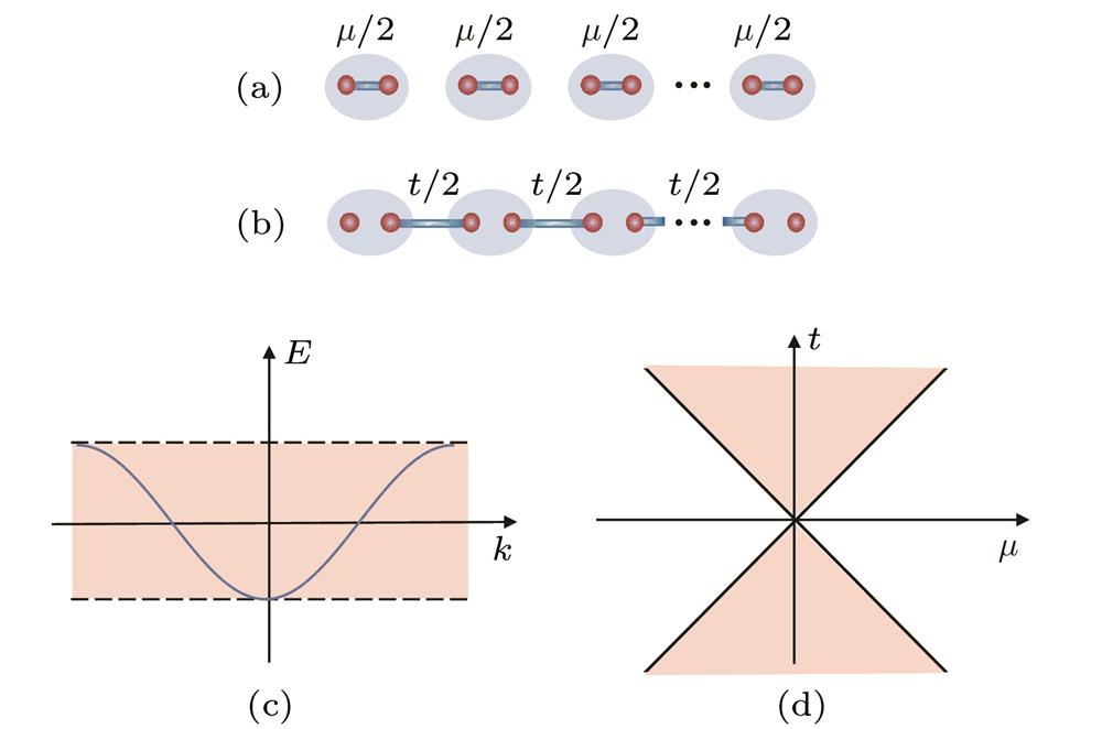
Fig. 1. Two topological phases of the Kiteaev chain. (a) Sche-matic illustration of the Hamiltonian in Majorana basis. In (a) , , only the first term survives thus Majoranas couple at the same site leaving no seperate MZMs left. In (b) , only the second term survives thus Majoranas couple at adjacent sites, leaving one MZM at each end of the chain. (c) Energy dispersion for . (d) Topological phase diagram of Kitaev chain. When the chemical potential crosses the nomal spectrum the system is in topological phase, as described by the orange region in (d); otherwise the system is trivial, as described by the white region in (d).

Fig. 2. Realizing MZMs in a 1D SOC nanowire^[8]. (a) Sketch of the basic setup. (b) Energy dispersion for the 1D SOC nanowire. When Zeeman field is absent, the system is time-reversal symmetric(TRS) and possesses even number of Fermi surfaces (red and blue curves); when Zeeman field is introduced, TRS is broken and a gap is opened at (black curves). Given that the chemical potential lies within gap, the system possesses only one Fermi surface, and the low-energy Hamilitonian is equivalent to that of the Kitaev chain. (c) Topological phase diagram of the system with the phase boundary given by . Orange (white) denotes topological (trivial) region.

Fig. 3. Skecth of a MZM braiding operation. (a) A system consists of 4 MZMs far enough apart, with and , and forming 2 fermions and . and are braided once clockwise. γ₂ crosses the branch cut of the votex hosting γ₃ and gains a minus sign, while γ₃ doesn't cross the branch cut of the votex hosting γ₂ and doesn't gain a minus sign. Hence the result is given by γ₂→ –γ₃, γ₃→ γ₂. (b) Worldlines in a space-time (x; t) diagram, describing four MZMs. and are braided once, hence their worldlines winds each other once. The initial state evolves into .

Fig. 4. Quantum gates realized by MZM braiding operations^[110]. (a)−(d) The elementary braids corresponding to the single-qubit gates H-, Z-gates on the first qubit as well as the 2-qubit CNOT and CZ gates.

Fig. 5. A T-junction allows for braiding process and the keyboard gates^[101]. The T-junction consists of two horizontal segments and one vertical segment. Dark blue segments are in topological phase, and light blue lines trivial phase. or is represented with rightward or upward pointing arrows, while or represents the leftward or downward pointing arrows. MZMs are transported according to the arrows around the T-junction. Black and gray blocks denote different states of tunable gates in accordance with trivial and topological phases. (a)–(d) sketch the process which is transported to vertical line firstly, then travels from the right end to the left end and at last is transported to the right end. After this process, the arrow points to the opposite direction. Local gates in (e) ensure that the MZMs can be manipulated gradually without closing the gap.

Fig. 6. Braiding operation via winding FI magnetization^[128]. (a) The monodromy operator can be realized by either braiding two MZMs or twisting each worldribbons by . The arrows indicate the MZM spin. The blue and red edges of the ribbon denote the evolution of internal degree of freedom. (b) MZMs in the SC/QSH/FI hybrid system. The yellow (red) arrows represent the directions of local spin polari-zations for MZMs (FI magnetization). Winding the red arrow at the bottom by , and are braided once; by they are braided twice. A reverse rotation leads to an inverse braiding operation.

Fig. 7. Basic set-up for qubit readout using a Josephson junction(JJ)^[129]. (a) The schematic of a JJ with 2 MZMs residing at the junction. The blue region denotes 1d TSC and the green denoted trivial insulator. The TSC region should be long enough so that the coupling of the MZMs through TSC is negligible. and couple weakly at the junction, forming a non-zero energy fermion. The phase difference can be varied by changing the magnetic flux . (b) The d.c. fractional Josephson current flowing across the junction versus . Instead of conventional -periodic JJ current induced by Cooper pair tunneling, the fractional JJ current induced by MZMs exhibits periodicity. The red dashed line denotes and the blue solid line denotes . The direction of the current is inverse for the qubit and , which enables the readout of the qubit by measuring the direct Josephson current.

Fig. 8. Sketch of MZMs coupled to quantum dots^[39], with 2-MZM and 4-MZM system shown in (a) and (b), and in (c) the local gates controlling the coupling between MZMs and quantum dots are shown.

Fig. 9. Majorana inferometry^[38]. (a) One path goes through two MZMs i.e. a topological qubit while the other path goes through a normal metal with a sufficiently long phase-coherence length. is the applied magnetic flux enclosed by the two paths. The phase difference of two paths is determined by the phase transition shift and the magnetic flux, which can be measured by the conductance. (b) Majorana interferometer provides a projective measurement of the fermion parity. Solid line and dotted line represent the conductance signals corresponding to qubits with parity 1 and –1 respectively.

Fig. 10. Time-reversal symmetry protected braiding process and the results of non-Abelian statistics^[156]. The TSC in (a) hosts a pair of MZMs at each end, and the braiding is fulfilled by the T-junction scheme. (b), (c) The evoluation of MKPs after the full braiding in the presence of different disorder strengh . The non-Abelian statistics is confirmed by . The adiabatic condition is satisfied in that .