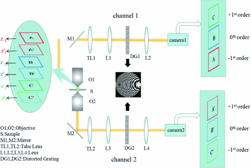
Fig. 1. Schematic diagram of DDBCM setup. The signal from particles in the sample (S) is collected by two identical objectives (O1, O2), resulting in two detection channels. In each channel, the signal passes through a tube lens (TL1 in channel 1 and TL2 in channel 2), then is modulated with a 4f relay system consisting of two lenses (L1 and L2 in channel 1 and L3 and L4 in channel 2), where a distorted grating (DG1 in channel 1 and DG2 in channel 2) is mounted at the Fourier plane, and is finally detected by a camera (camera 1 in channel 1 and camera 2 in channel 2). As is shown in the enlarged sample area, three focal planes at depths z1, z2, and z3, denoted by capital letters A, B, and C for channel 1 (or at depths z1′, z2′, and z3′, denoted by capital letters A′, B′, and C′ for channel 2) separated by 4 μm are simultaneously imaged in three different areas, corresponding to three different diffraction orders. In channel 1, A, B, and C are simultaneously imaged on camera 1, while A′, B′, and C′ in channel 2 are simultaneously imaged on camera 2.

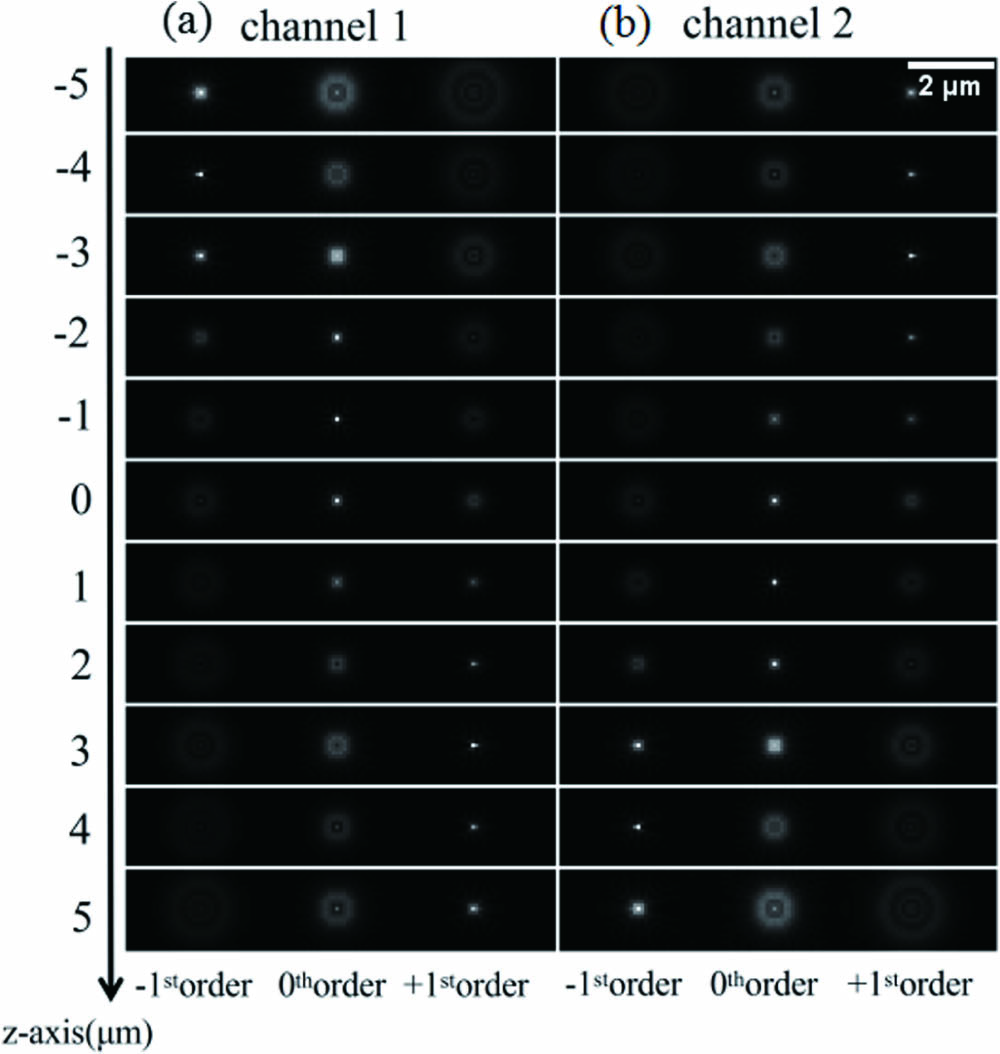
Fig. 2. Images of a single particle at 11 axial positions, from z=−5μm to z=5μm. At each axial position, the particle is imaged in six areas, corresponding to three sub-imaging areas for the −1st, 0th, and +1st diffraction orders in channel 1 and three other ones in channel 2. No matter where the particle is, it can be always captured in certain sub-images in the two channels.

Fig. 3. Two trajectories of two particles. (a) Trajectories of P1 (bottom-up) and P2 (top-down) with time coding by the pseudo-color. (b) Three pairs of images at three time points, t=0s, 2.5 s, 5.0 s. For each particle, the image in each channel consists of three sub-images, which are from three different diffraction orders, respectively, and two appropriate sub-images are chosen for subsequent localization. The sub-images chosen for localization at the three time points are shown in blue and red circles.

Fig. 4. Localization precision analysis of DDBCM. (a) 3D trajectories of the two particles, whose localizations were measured every 0.1 s from t=0s to t=10s, and the result localizations are shown with small circles. (b) Statistical localization precision along three directions. Gaussian fitting to the distribution of localization discrepancy of P1 at 101 time points demonstrated that the localization precisions in the x, y, and z axes are 4.5 nm, 4.3 nm, and 17.1 nm, respectively. (c) Lateral (x and y) and axial (z) localization precisions of the same particle throughout a depth range of 10 μm with the SNR set to 30 dB. (d) Localization precision in the x, y, and z axes of the same particle at z=0μm as a function of SNR.

Fig. 5. Comparison of the (a) lateral and (b) axial localization precision and (c) the capability of 3D localization for the DDBCM approach, the biplane approach, and the DSBCM approach, whose detection strategies are shown in the left column. In all cases, each objective is assumed to collect 3000 photons for each particle, all these photons are evenly assigned to each sub-image, and the background level is set to 2 photons/pixel.

Table 1. Sub-images Chosen for 3D Localization Algorithm for Different Depth Ranges