Abstract
Tracking moving particles in cells by single particle tracking is an important optical approach widely used in biological research. In order to track multiple particles within a whole cell simultaneously, a parallel tracking approach with large depth of field was put forward. It was based on distorted grating and dual-objective bifocal imaging, making use of the distorted grating to expand the depth of field, dual-objective to gather as many photons as possible, and bifocal plane imaging to realize three-dimensional localization. Simulation of parallel tracking of two particles moving along the z axis demonstrated that even when the two are axially separated by 10 μm, they can both be localized simultaneously with transversal precision better than 5 nm and axial precision better than 20 nm.The study of life processes at the cellular and molecular level is of great significance to understand biological systems and fight diseases. For vesicles and other moving targets, single particle tracking (SPT) is a powerful optical tool, which can be used to analyze the behavior of these individual particles with high localization precision. So far, several approaches for three-dimensional (3D) SPT have been reported, by means of astigmatism (cylindrical lens)[1], double-helix point spread function (DH-PSF)[2–4], self-bend PSF (SB-PSF)[5,6], self-interference PSF (SELFI)[7], or some other approaches based on PSF engineering[8–13]. However, these engineered PSFs are sensitive to optical aberrations, so localization precision in the axis has to be sacrificed for larger effective depth of field (DOF), which is the requirement for tracking particles in a whole cell with 10 μm in thickness. In order to track particles in a whole cell, these 3D localization methods must be combined with some approaches to extend DOF[14–19]. DOF stacking is a common method, such as multifocal plane microscopy (MUM)[20], where multiple planes at different depths are imaged with multiple detectors. Another strategy is axial scanning to extend DOF, but it is obviously time consuming, which is not optimal for dynamic imaging. Furthermore, information in one certain plane will be lost between adjacent scans. In a previous study, an aberration-corrected multifocus microscopy (MFM) has demonstrated an impressive axial tracking range, which uses a focal stack to yield nine two-dimensional images[21]. Nine images, however, mean that only one-ninth of the photons collected per particle are assigned per image, which decreases the localization precision accordingly. In order to make full use of the photons emitted from particles, two objectives can be used, which is also the strategy adopted in 4Pi microscopy. In 4Pi microscopy, fluorescence emission from a single molecule is collected with two objectives, and then they interfere at the detector, so there is a significant improvement in axial localization precision over single objective approaches[22,23]. However, because of the unique features of the interference pattern, this interference method was initially restricted to very thin samples, such as 250 nm in thickness[22], later to 700–1000 nm[24,25]. More recently, cells as thick as 10 μm were successfully imaged with an updated 4Pi configuration named whole cell 4Pi single molecule switching nanoscopy (W-4PiSMSN)[26]. But, for samples thicker than 1.2 μm, the sample stage should be translated axially in 500 nm steps to acquire the information for the whole targeted imaging volume.
Here, we present an image-based tracking method for simultaneously tracking multiple particles in a whole cell as thick as 10 μm, which means that no sample stage translation will be necessary. The method is called distorted grating (DG) and dual-objective bifocal plane combination microscopy (DDBCM). In DDBCM, photons collected from each particle are doubled, which improves the localization precision by ∼1.4 fold in all three dimensions, and totally six different focal planes are captured simultaneously, so with a reasonable arrangement of these six focal planes, effective DOF would be six fold that of traditional single plane microscopes and three fold that of bifocal plane microscopy (biplane). Particles in the effective DOF are localized in three dimensions with the bifocal localization algorithm[27–30]. With DDBCM, multiple particles in a whole cell can be localized simultaneously, and a nanometric localization precision in the axial range of 10 μm can be achieved.
The strategy for image detection is shown in Fig. 1. Dual-objective configuration (O1 and O2) is implemented, so there are two detection channels. Photons collected from each particle are doubled because of the dual-objective configuration, so theoretically times better localization precision can be expected accordingly, since the localization precision is dependent on the number of photons[31–33]. For each detection channel, thanks to the DGs (denoted by DG1 and DG2 in Fig. 1), three focal planes at depths , , and , denoted by capital letters A, B and C for channel 1 (or at depths , , and , denoted by , , and for channel 2) separated by 4 μm are imaged simultaneously. Furthermore, the three focal planes of one detection channel are staggered from the other three focal planes of the other channel, and thus 3D high localization precision at an axial range of 10 μm can be achieved by the bifocal localization algorithm. In fact, a phase mask of the DG is an off-axis Fresnel zone plate[34–37], producing positive focusing power in positive diffraction orders and negative focusing power in negative diffraction orders, and leaving the zeroth diffraction order unchanged. This modification enables different diffraction orders to image multiple object planes side-by-side on one camera. Similarly, we can get three different diffraction order sub-images in the other channel. According to the specific depth of the particle, sub-images from appropriate diffraction orders in two channels can be chosen as source images for localization.
Sign up for Chinese Optics Letters TOC. Get the latest issue of Chinese Optics Letters delivered right to you!Sign up now

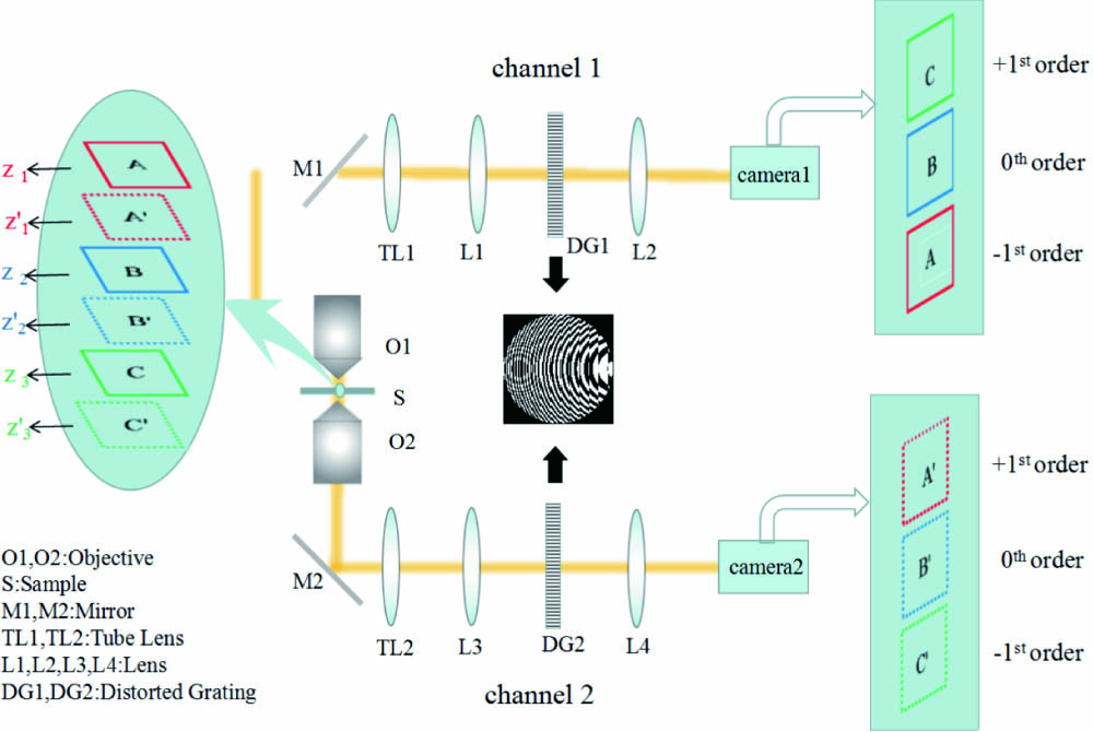
Figure 1.Schematic diagram of DDBCM setup. The signal from particles in the sample (S) is collected by two identical objectives (O1, O2), resulting in two detection channels. In each channel, the signal passes through a tube lens (TL1 in channel 1 and TL2 in channel 2), then is modulated with a relay system consisting of two lenses (L1 and L2 in channel 1 and L3 and L4 in channel 2), where a distorted grating (DG1 in channel 1 and DG2 in channel 2) is mounted at the Fourier plane, and is finally detected by a camera (camera 1 in channel 1 and camera 2 in channel 2). As is shown in the enlarged sample area, three focal planes at depths , , and , denoted by capital letters A, B, and C for channel 1 (or at depths , , and , denoted by capital letters , , and for channel 2) separated by 4 μm are simultaneously imaged in three different areas, corresponding to three different diffraction orders. In channel 1, A, B, and C are simultaneously imaged on camera 1, while , , and in channel 2 are simultaneously imaged on camera 2.
We simulate the imaging process of DDBCM. In all simulations, the emission wavelengths of particles are set to 560 nm. Two identical oil immersion objectives (NA 1.4, 100×) are used to collect emission signals. The detection path for each channel is the same. As is shown in Fig. 1, the DG phase mask is placed on the Fourier plane of a relay system consisting of two 200 mm lenses (L1 and L2 for channel 1, and L3 and L4 for channel 2). The signal is finally detected with two detectors with a pixel size of 16 μm, twice that of the pixelized phase mask.
In the first simulation, a particle at different axial positions is imaged in two detection channels, respectively. The midpoint of the two opposing objectives is set to the zero depth, i.e., . The particle at eleven different depths ranging from to is imaged by the two channels, and, for each one, there are three sub-images corresponding to the three diffraction orders, respectively, as shown in Fig. 2. For a particle in a certain depth range, two certain sub-images are chosen for the dual-focal localization algorithm. Since there are a total of six sub-images for a particle, there are five combinations for five different depth ranges, and each combination is effective for localizing particles in a certain depth range of 2 μm, as is shown in Table 1. For example, when the particle is in the depth range of , the diffraction order sub-image in channel 1 [see Fig. 2(a)] and the diffraction order sub-image in channel 2 [see Fig. 2(b)] are chosen for localization, which means that the two diffraction orders are equivalent to two planes of bifocal imaging.
Figure 2.Images of a single particle at 11 axial positions, from to . At each axial position, the particle is imaged in six areas, corresponding to three sub-imaging areas for the , , and diffraction orders in channel 1 and three other ones in channel 2. No matter where the particle is, it can be always captured in certain sub-images in the two channels.
| Depth Ranges (μm) | Channel 1 | Channel 2 |
|---|
| −5–−3 | −1st order | +1st order |
| −3–−1 | +1st order | 0th order |
| −1–1 | 0th order | 0th order |
| 1–3 | 0th order | +1st order |
| 3–5 | +1st order | −1st order |
Table 1. Sub-images Chosen for 3D Localization Algorithm for Different Depth Ranges
In the next simulation, two moving particles (P1 and P2) are traced. The initial 3D positions of P1 and P2 are set to (, 7, ) and (2, , 5) (in μm), respectively. P1 moves from the bottom to top along the spiral trajectory described as (, , ) (in μm), and P2 moves from top to bottom along the spiral trajectory described as (, , ), as shown with the pseudo-color plot in Fig. 3(a). Images of the two particles at three different times (, , ) are shown in Fig. 3(b). In the very beginning (), P1 and P2 are at depths of and 5 μm, respectively, which means that the two particles are 10 μm apart in the axis. With time increasing, P1 and P2 move closer to each other until , when two particles are at the zero depth, so the two images from two channels are almost the same because of the symmetry of these two detection channels. Thereafter, two particles are apart from each other until two particles finally go back to the original lateral positions, but their axial positions are interchanged. Totally, from to , 202 images from two channels at 101 time points were recorded with a time interval of 0.1 s, which means that the two particles move 0.1 μm in the axis in adjacent frames. For each single particle, 1000 fluorescence photons are assumed to be collected in each sub-image. Considering real scenarios, images are always deteriorated by inevitable Poisson noise derived from independence of photon detections and some Gaussian noises, which are hard to avoid, such as background noise and readout noise; so, in order to make the images more practical, Poisson and Gaussian noises are added, and the best signal-to-noise ratio (SNR) of the images from two channels is set to 30, which means the background noise added is 3 photons/pixel. Here, , where the signal is the maximum intensity of the 202 images, and the noise is the standard deviation (STD) of background noise added[5]. Two source images for localization of P1 and P2 are highlighted with blue and red circles, respectively.
Figure 3.Two trajectories of two particles. (a) Trajectories of P1 (bottom-up) and P2 (top-down) with time coding by the pseudo-color. (b) Three pairs of images at three time points, , 2.5 s, 5.0 s. For each particle, the image in each channel consists of three sub-images, which are from three different diffraction orders, respectively, and two appropriate sub-images are chosen for subsequent localization. The sub-images chosen for localization at the three time points are shown in blue and red circles.
Next, based on the simulated images, we select appropriate sub-images from two detection channels for the localization algorithm[27,28], then P1 and P2 at 101 different time points are localized [see Fig. 4(a)], and the localizations fit well with their true positions. In particular, the localization precision along three dimensions is analyzed quantitatively based on the data of 101 localizations for one particle at 101 different depths. The result after Gaussian fitting to the distribution of localization discrepancy in three dimensions shows that the corresponding average localization precision of the , , and axes is 4.5 nm, 4.3 nm, and 17.1 nm (STD), respectively [Fig. 4(b)]. The axial localization precision is confined in for the whole axial range of 10 μm, while the lateral localization precision is much better and more constant, as is shown in Fig. 4(c). To further assess the localization capability of DDBCM at different noise levels, with an assumption that the particle is at , we measure the 3D localization precision at six SNRs, where the data for statistics come from 100 measurements. As is shown in Fig. 4(d), localization precision improves with increasing SNR. For an SNR of 33 dB, an axial precision of better than 10 nm was recorded.
Figure 4.Localization precision analysis of DDBCM. (a) 3D trajectories of the two particles, whose localizations were measured every 0.1 s from to , and the result localizations are shown with small circles. (b) Statistical localization precision along three directions. Gaussian fitting to the distribution of localization discrepancy of P1 at 101 time points demonstrated that the localization precisions in the , , and axes are 4.5 nm, 4.3 nm, and 17.1 nm, respectively. (c) Lateral ( and ) and axial () localization precisions of the same particle throughout a depth range of 10 μm with the SNR set to 30 dB. (d) Localization precision in the , , and axes of the same particle at as a function of SNR.
Finally, we analyzed the best possible localization precision that DDBCM could achieve and compared that with two other MUM approaches using a single objective. In one of approaches, there are also two detection channels whose focal planes are separated by 2 μm (see the detection strategy denoted by Biplane in Fig. 5), so there are two sub-images for each particle. The other approach is a kind of DG and single objective bifocal plane combination microscopy [see the detection strategy denoted by dual-objective bifocal plane combination microscopy (DSBCM) in Fig. 5], and the difference between the Biplane and the DSBCM is that there is a relay system in DSBCM, with a DG at the Fourier plane, inserted after the tube lens, which is the same as that used in DDBCM, so there are six sub-images for each particle.
Figure 5.Comparison of the (a) lateral and (b) axial localization precision and (c) the capability of 3D localization for the DDBCM approach, the biplane approach, and the DSBCM approach, whose detection strategies are shown in the left column. In all cases, each objective is assumed to collect 3000 photons for each particle, all these photons are evenly assigned to each sub-image, and the background level is set to 2 photons/pixel.
Theoretical localization precision can be achieved by an unbiased estimator of the PSF. In all cases, a single objective was assumed to collect 3000 photons from one particle. So, for the DDBCM, 1000 photons are assumed to be collected in each sub-image, while 500 photons are collected for the DSBCM. For the Biplane, 1500 photons can be assigned to each plane, and the background level is set to 2 photons/pixel. The performance of different tracking approaches is compared and analyzed by means of Cramer–Rao bound (CRB), which is the inverse of the Fisher information matrix. Their lateral ( and ) and axial () localization precision and the capability of 3D localization (the square root of 3D localization precision) as functions of the axial position are shown in Fig. 5. The behaviors of the localization precision for the DDBCM and DSBCM are similar but significantly different from that for the Biplane. The localization precision for the Biplane in the depth range around the zero depth () is higher than that for the DDBCM and the DSBCM, but then deteriorates dramatically beyond this axial range, while that localization precision for the DDBCM and DSBCM is more constant for all depths [Figs. 5(a) and (b)]. As to the DDBCM and the DSBCM, the localization precision for the former is noticeably better than that for the latter, which is reasonable because two times the photons are collected for the DDBCM. The capability of 3D localization shows similar results [Fig. 5(c)].
In summary, we present a novel method, DDBCM, for multiparticle parallel tracking with nanometric localization precision in three dimensions and extended DOF as large as 10 μm. It combines the DOF extension ability of DGs and 3D localization ability of the bifocal detection method; furthermore, photons collected from single particles are doubled because of the dual-objective configuration. The simulations demonstrate that our method can be used to track multiple particles in the axial range of 10 μm simultaneously, with nanometric localization precision. The implementation of the DDBCM should not be a problem since bifocal imaging by positioning two microscopes opposite to each other has been achieved in Ref. [31]. In this Letter, only one-dimensional DGs are discussed. Actually, the DOF can be further extended by using a two-dimensional DG[21,37], which, however, will decrease the SNR of the raw image because fixed photons have to be divided into more parts. Generally, the phase mask of DGs can be implemented with a spatial light modulator, which will cause the loss of photons. So, in order to avoid unnecessary loss of photons, a phase mask with a fixed pattern can be fabricated by gray-level lithography.
References
[1] B. Huang, W. Wang, M. Bates, X. Zhuang. Science, 319, 810(2008).
[2] S. R. P. Pavani, A. Greengard, R. Piestun. Appl. Phys. Lett., 95, 021103(2009).
[3] S. R. P. Pavani, M. A. Thompson, J. S. Biteen, S. J. Lord, N. Liu, R. J. Twieg, R. Piestun, W. E. Moerner. Proc. Natl. Acad. Sci. USA, 106, 2995(2009).
[4] S. R. P. Pavani, R. Piestun. Opt. Express, 16, 22048(2008).
[5] Y. Zhou, P. Zammit, G. Carles, A. R. Harvey. Opt. Express, 26, 7563(2018).
[6] S. Jia, J. C. Vaughan, X. Zhuang. Nat. Photon., 8, 302(2014).
[7] P. Bon, J. Linarès-Loyez, M. Feyeux, K. Alessandri, B. Lounis, P. Nassoy, L. Cognet. Nat. Methods, 15, 449(2018).
[8] C. Manzo, M. F. Garcia-Parajo. Rep. Prog. Phys., 78, 124601(2015).
[9] W. Liu, K. C. Toussaint, C. Okoro, D. Zhu, Y. Chen, C. Kuang, X. Liu. Laser Photon. Rev., 12, 1700333(2018).
[10] A. von Diezmann, Y. Shechtman, W. E. Moerner. Chem. Rev., 117, 7244(2017).
[11] A. S. Backer, M. P. Backlund, A. R. von Diezmann, S. J. Sahl, W. E. Moerner. Appl. Phys. Lett., 104, 193701(2014).
[12] C. Roider, A. Jesacher, S. Bernet, M. Ritsch-Marte. Opt. Express, 22, 4029(2014).
[13] A. Aristov, B. Lelandais, E. Rensen, C. Zimmer. Nat. Commun., 9, 2409(2018).
[14] D. Chen, B. Yu, H. Li, Y. Huo, B. Cao, G. Xu, H. Niu. Opt. Lett., 38, 3712(2013).
[15] Y. Shechtman, L. E. Weiss, A. S. Backer, S. J. Sahl, W. E. Moemer. Nano Lett., 15, 4194(2015).
[16] M. Duocastella, C. Theriault, C. B. Arnold. Opt. Lett., 41, 863(2016).
[17] G. Sancataldo, L. Scipioni, T. Ravasenga, L. Lanzano, A. Diaspro, A. Barberis, M. Duocastella. Optica, 4, 367(2017).
[18] Z. Cheng, H. Ma, Z. Wang, S. Yang. Chin. Opt. Lett., 16, 081701(2018).
[19] D. Wang, Y. Meng, D. Chen, Y. Yam, S. Chen. Chin. Opt. Lett., 15, 090004(2017).
[20] P. Prabhat, S. Ram, E. S. Ward, R. J. Ober. Proc. SPIE, 6090, 60900L(2006).
[21] S. Abrahamsson, J. Chen, B. Hajj, S. Stallinga, A. Y. Katsov, J. Wisniewski, G. Mizuguchi, P. Soule, F. Mueller, C. D. Darzacq, X. Darzacq, C. Wu, C. I. Bargmann, D. A. Agard, M. Dahan, M. G. L. Gustafsson. Nat. Methods, 10, 60(2013).
[22] G. Shtengel, J. A. Galbraith, C. G. Galbraith, J. Lippincott-Schwartz, J. M. Gillette, S. Manley, R. Sougrat, C. M. Waterman, P. Kanchanawong, M. W. Davidson, R. D. Fetter, H. F. Hess. Proc. Natl. Acad. Sci. USA, 106, 3125(2009).
[23] Z. Gu, X. Wang, J. Wang, F. Fan, S. Chang. Chin. Opt. Lett., 17, 121103(2019).
[24] D. Aquino, A. Schonle, C. Geisler, C. V. Middendorff, C. A. Wurm, Y. Okamura, T. Lang, S. W. Hell, A. Egner. Nat. Methods, 8, 353(2011).
[25] T. A. Brown, A. N. Tkachuk, G. Shtengel, B. G. Kopek, D. F. Bogenhagen, H. F. Hess, D. A. Clayton. Mol. Cell. Biol., 31, 4994(2011).
[26] F. Huang, G. Sirinakis, E. S. Allgeyer, L. K. Schroeder, W. C. Duim, E. B. Kromann, T. Phan, F. E. Rivera-Molina, J. R. Myers, I. Irnov, M. Lessard, Y. Zhang, M. A. Handel, C. Jacobs-Wagner, C. P. Lusk, J. E. Rothman, D. Toomre, J. Booth, J. Bewersdorf. Cell, 166, 1028(2016).
[27] S. Ram, P. Prabhat, J. Chao, E. S. Ward, R. J. Ober. Biophys. J., 95, 6025(2008).
[28] E. Toprak, H. Balci, B. H. Blehm, P. R. Selvin. Nano. Lett., 7, 2043(2007).
[29] M. Speidel, A. Jonas, E. L. Florin. Opt. Lett., 28, 69(2003).
[30] R. Velmurugan, J. Chao, S. Ram, E. S. Ward, R. J. Ober. Opt. Express, 25, 3394(2017).
[31] S. Ram, P. Prabhat, E. S. Ward, R. J. Ober. Opt. Express, 17, 6881(2009).
[32] R. J. Ober, S. Ram, E. S. Ward. Biophys. J., 86, 1185(2004).
[33] R. E. Thompson, D. R. Larson, W. W. Webb. Biophys. J., 82, 2775(2002).
[34] P. M. Blanchard, A. H. Greenaway. Opt. Commun., 183, 29(2000).
[35] P. A. Dalgarno, H. I. Dalgarno, A. Putoud, R. Lambert, L. Paterson, D. C. Logan, D. P. Towers, R. J. Warburton, A. H. Greenaway. Opt. Express, 18, 877(2010).
[36] P. M. Blanchard, D. J. Fisher, S. C. Woods, A. H. Greenaway. Appl. Opt., 39, 6649(2000).
[37] P. M. Blanchard, A. H. Greenaway. Appl. Opt., 38, 6692(1999).