Infrared and Visible Image Fusion Method Based on Tikhonov Regularization and Detail Reconstruction

Xin Lu; Lin Yang; Min Li; Xuewu Zhang

doi:10.3788/AOS202040.0210001

Journals >Acta Optica Sinica >Volume 40 >Issue 2 >Page 0210001 > Article

Acta Optica Sinica
Vol. 40, Issue 2, 0210001 (2020)

Infrared and Visible Image Fusion Method Based on Tikhonov Regularization and Detail Reconstruction

Xin Lu, Lin Yang, Min Li, and Xuewu Zhang^*

Author Affiliations

College of Internet of Things Engineering, Hohai University, Changzhou, Jiangsu 213022, China

show less

DOI: 10.3788/AOS202040.0210001 Cite this Article Set citation alerts

Xin Lu, Lin Yang, Min Li, Xuewu Zhang. Infrared and Visible Image Fusion Method Based on Tikhonov Regularization and Detail Reconstruction[J]. Acta Optica Sinica, 2020, 40(2): 0210001 Copy Citation Text

show less

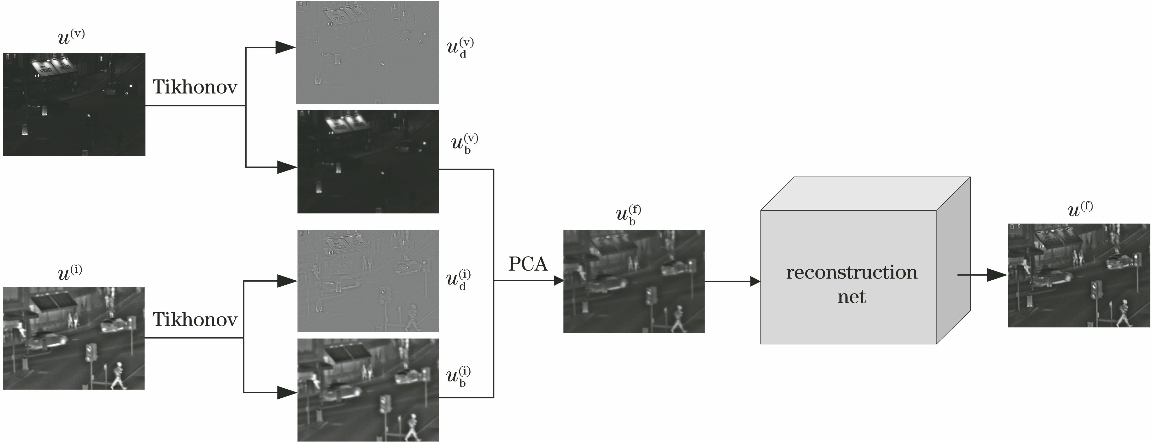
Fig. 1. Algorithm flow diagram

Download full size

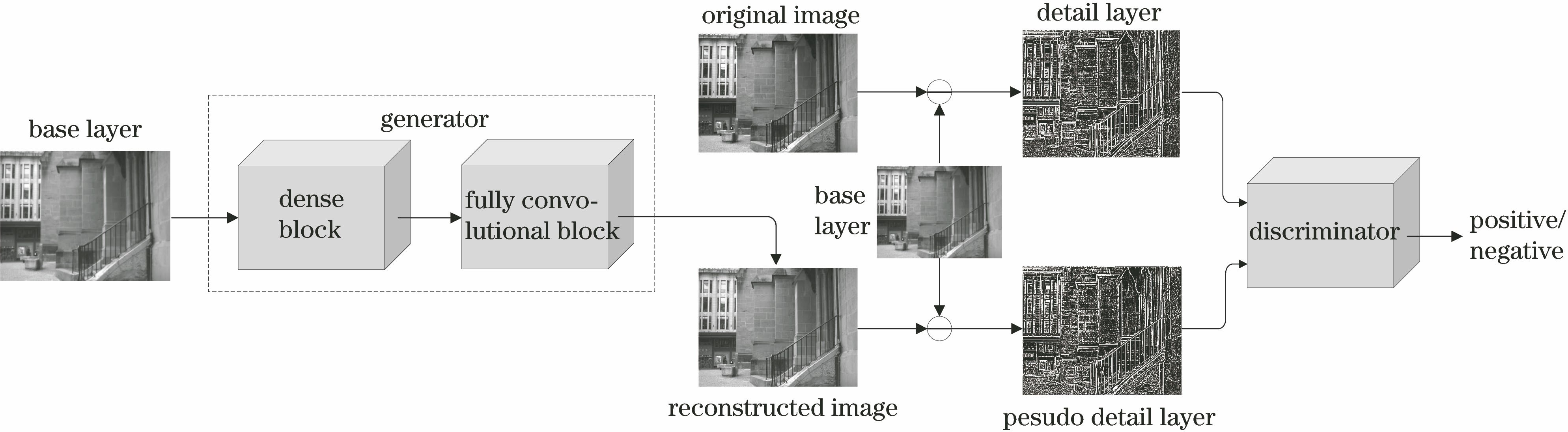
Fig. 2. Framework of image reconstruction model

Download full size

Fig. 3. Generative network structure

Download full size

Fig. 4. Discriminant network structure

Download full size

Fig. 5.

Network training process

Download full size

Fig. 6. Comparison of decomposition effects of different decomposition algorithms for “Smoke” scene. (a) Original image; (b) bilateral filtering; (c) guided filtering; (d) Gaussian pyramid; (e) wavelet transform; (f) Tikhonov regularization, α=2; (g) Tikhonov regularization, α=4 ; (h) Tikhonov regularization, α=8

Download full size

Fig. 7. Comparison of decomposition effects of different decomposition algorithms for “Heather” scene. (a) Original image; (b) bilateral filtering; (c) guided filtering; (d) Gaussian pyramid; (e) wavelet transform; (f) Tikhonov regularization, α=2; (g) Tikhonov regularization, α=4 ; (h) Tikhonov regularization, α=8

Download full size

Fig. 8. Fusion effects of different algorithms in “Quad” scene. (a) Visible image; (b) infrared image; (c) DenseNet; (d) LatLRR; (e) VGG; (f) ResNet; (g) VSM; (h) QD; (i) GAN; (j) proposed algorithm

Download full size

Fig. 9. Fusion effects of different algorithms in “Smoke” scene. (a)Visible image; (b) infrared image; (c) DenseNet; (d) LatLRR; (e) VGG;(f) ResNet; (g) VSM; (h) QD; (i) GAN; (j) proposed algorithm

Download full size

Fig. 10. Fusion effects of different algorithms in “Nato_camp” scene. (a) Visible image; (b) infrared image; (c) DenseNet; (d) LatLRR; (e) VGG; (f) ResNet; (g) VSM; (h) QD; (i) GAN; (j) proposed algorithm

Download full size

Fig. 11. Fusion effects of different algorithms in blurred “Kaptein_1123” scene. (a) Visible image; (b) infrared image; (c) DenseNet; (d) LatLRR; (e) VGG; (f) ResNet; (g) VSM; (h) QD; (i) GAN; (j) proposed algorithm

Download full size

Fig. 12. Fusion effects of different algorithms in blurred “Heather” scene. (a) Visible image; (b) infrared image; (c) DenseNet; (d) LatLRR; (e) VGG; (f) ResNet; (g) VSM; (h) QD; (i) GAN; (j) proposed algorithm

Download full size

Fig. 13. Fusion results of proposed algorithm in other scenes. (a) Steamer; (b) Bunker; (c) Street; (d) Jeep; (e) Soldier

Download full size

Fig. 14. Comparison of program running time of different algorithms

Download full size

Name	Kernel size	Stride	Padding	Output padding	Output size	BN
Input	-	-	-	-	320×320×64	-
Conv1	128×5×5	2	2	-	160×160×128	√
Conv2	256×3×3	2	1	-	80×80×256	√
Conv3	512×3×3	2	1	-	40×40×512	√
Conv4	512×3×3	2	1	-	20×20×512	√
Conv5	1024×1×1	2	-	-	10×10×1024	√
DeConv1	512×1×1	2	-	1	20×20×512	√
Add(Conv4+DeConv1)	-	-	-	-	20×20×512	-
DeConv2	512×1×1	2	1	1	40×40×512	√
Add(Conv3+DeConv2)	-	-	-	-	40×40×512	-
DeConv3	256×3×3	2	1	1	80×80×256	√
Add(Conv2+DeConv3)	-	-	-	-	80×80×256	-
DeConv4	128×3×3	2	1	1	160×160×128	√
Add(Conv1+DeConv4)	-	-	-	-	160×160×128	-
DeConv5	64×5×5	2	2	1	320×320×64	√
Add(Input+DeConv5)	-	-	-	-	320×320×64	-
Output	1×5×5	1	2	-	320×320×1	-

Table 1. Parameter information of fully convolutional block

Image	Metric	DenseNet	LatLRR	VGG	ResNet	VSM	QD	GAN	Proposed method
Bunker	EN	6.9807	6.8143	6.7277	6.8048	7.1073	7.0720	6.7043	7.1513
	SD	31.403	28.379	26.137	28.186	36.006	39.471	25.947	37.497
	SSIM	1.2790	1.1806	1.1504	1.1850	1.2137	1.0272	1.1479	1.1767
	CC	0.6270	0.6316	0.6345	0.6397	0.6223	0.5394	0.6326	0.6274
	SF	0.0180	0.0198	0.0202	0.0203	0.0213	0.0209	0.0212	0.0213
Heather	EN	6.9413	6.6036	6.8643	6.7372	7.1234	6.7995	6.7411	7.0281
	SD	32.674	26.337	30.489	28.537	38.267	31.185	30.191	37.529
	SSIM	1.0185	0.9573	1.0136	1.0044	1.0434	0.8266	0.9095	0.9770
	CC	0.5575	0.5574	0.5649	0.5680	0.5380	0.4624	0.5106	0.5545
	SF	0.0174	0.0186	0.0197	0.0194	0.0210	0.0191	0.0204	0.0212
Sandpath	EN	6.7642	6.2525	6.5866	6.5419	6.5419	6.7348	6.1159	6.7899
	SD	29.812	22.357	26.159	27.952	27.952	32.385	18.072	28.921
	SSIM	0.9022	0.8195	0.8885	0.8811	0.8811	0.8018	0.7723	0.8921
	CC	0.4780	0.4733	0.4858	0.4681	0.4681	0.4286	0.4816	0.4725
	SF	0.0268	0.0262	0.0269	0.0273	0.0273	0.0270	0.0269	0.0273
Jeep	EN	7.1496	6.5470	7.1331	6.9949	7.0240	7.2358	6.7980	7.2032
	SD	35.988	23.430	35.080	33.683	35.427	39.738	28.669	38.340
	SSIM	0.6512	0.5018	0.6460	0.6288	0.6322	0.5875	0.4970	0.6019
	CC	0.3641	0.3617	0.3650	0.3671	0.3553	0.3174	0.2818	0.3428
	SF	0.0132	0.0129	0.0151	0.0151	0.0161	0.0158	0.0152	0.0170

Table 2. Objective evaluation results of different fusion methods

Xin Lu, Lin Yang, Min Li, Xuewu Zhang. Infrared and Visible Image Fusion Method Based on Tikhonov Regularization and Detail Reconstruction[J]. Acta Optica Sinica, 2020, 40(2): 0210001

Download Citation

Set citation alerts for the article

Tools

Set citation alerts for the article

Save the article for my favorites

Paper Information