• Photonics Research
  • Vol. 9, Issue 7, 1300 (2021)
Arutyun Bagramyan1、2、4、*, Loïc Tabourin1、2, Ali Rastqar2, Narges Karimi2, Frédéric Bretzner2、3、5、*, and Tigran Galstian1、6、*
Author Affiliations
  • 1Center for Optics, Photonics and Lasers (COPL), Faculty of Science and Engineering, Department of Physics, Engineering Physics and Optics, Université Laval, Québec, QC G1V 0A6, Canada
  • 2Centre de Recherche du CHU de Québec-Université Laval, CHUL-Neurosciences, Québec, QC G1V 4G2, Canada
  • 3Department of Psychiatry and Neurosciences, Faculty of Medicine, Université Laval, Québec, QC G1V 0A6, Canada
  • 4e-mail: arutyun.bagramyan.1@ulaval.ca
  • 5e-mail: frederic.bretzner.1@ulaval.ca
  • 6e-mail: tigran.galstian@phy.ulaval.ca
  • show less
    DOI: 10.1364/PRJ.418154 Cite this Article Set citation alerts
    Arutyun Bagramyan, Loïc Tabourin, Ali Rastqar, Narges Karimi, Frédéric Bretzner, Tigran Galstian. Focus-tunable microscope for imaging small neuronal processes in freely moving animals[J]. Photonics Research, 2021, 9(7): 1300 Copy Citation Text show less
    Liquid crystal lens schematics and characterization. (a) Schematic demonstration of the structure of the TLCL used (see the main text for details). WCL, weakly conductive layer; PI, polyimide alignment layer; HPE, hole patterned electrode; TA, transparent adhesive; and U-ITO, uniform ITO electrode. The distribution of the electrical field is shown by the black arrows within the LC layer. (b) Control of the focal distance of the TLCL by the frequency of the excitation electrical signal (AC square shaped, at 3VRMS) and corresponding RMS aberrations.
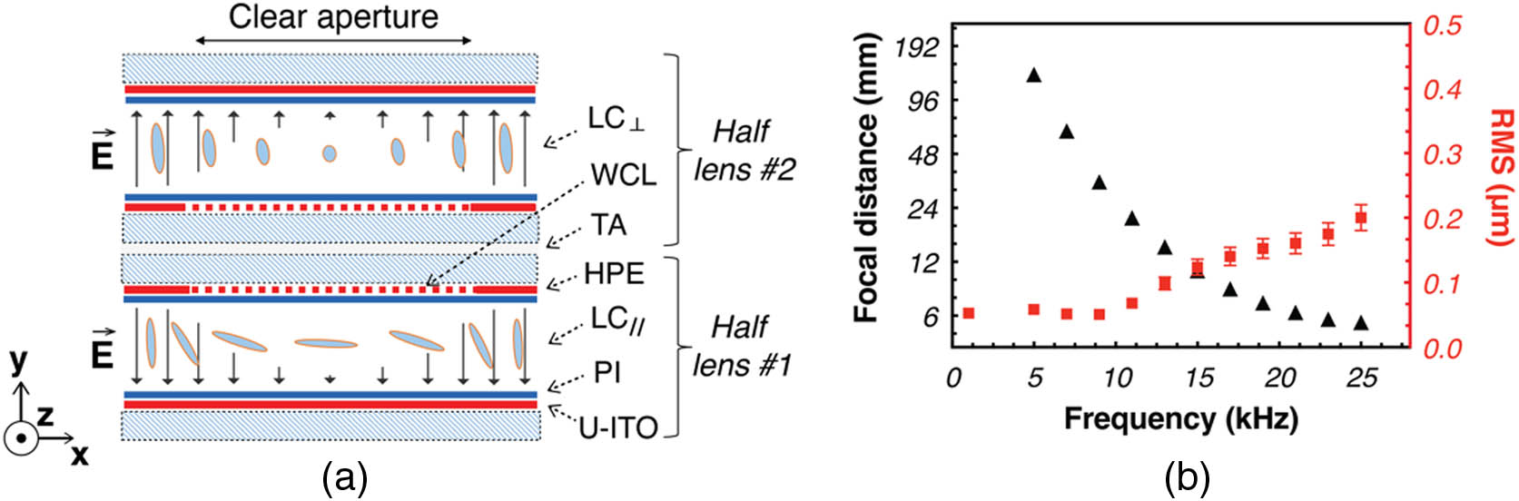
    Fig. 1. Liquid crystal lens schematics and characterization. (a) Schematic demonstration of the structure of the TLCL used (see the main text for details). WCL, weakly conductive layer; PI, polyimide alignment layer; HPE, hole patterned electrode; TA, transparent adhesive; and U-ITO, uniform ITO electrode. The distribution of the electrical field is shown by the black arrows within the LC layer. (b) Control of the focal distance of the TLCL by the frequency of the excitation electrical signal (AC square shaped, at 3VRMS) and corresponding RMS aberrations.
    Schematic presentation of the ensemble of the imaging system. (a) Schematic of the system: 1, extension cable for the CMOS; 2, TLCL wires; 3, optical fiber; 4, light source; 5, DAQCMOS; 6, rotary joint system; 7, LED driver; 8, DAQLabVIEW; 9, camera to record behavior; and 10, LabVIEW user interface. (b) Photo of the TLCL within the mDS1s. (c) Electrically induced focal shift of the mDS1s simulated using Zemax optical software. Experimental results were obtained by measuring the FWHM of the point spread function of 1 μm diameter fluorescence. Error bars correspond to the standard deviation. (d) Schematic representation of optical components. Light from the optical fiber is first collimated by a large-diameter GRIN lens and then reflected by the 45° prism. The excitation filter is used to preserve the desired wavelengths and the dichroic mirror to reflect light into the plano-convex lens, toward the TLCL. Excitation light is then guided within the optical probe assembly to finally reach the object/structure of interest. The emission (fluorescent) light passes back through the probe to reach first the TLCL and then the plano-convex lens. The latter focuses the image on the CMOS sensor passing first through the dichroic mirror and the emission filter. (e) Schematic side view of the optical probe with three components: 45° prism, imaging (NA = 0.42), and rod GRIN (NA = 0.2) lenses. (f) Displacement path of the animal during the portability test (≈4 min). AnimalTracker plug-in (ImageJ) was used to track and analyze the animal’s movement. (g) Total traveled distance. (h) Average moving speed. Error bars correspond to the standard deviation.
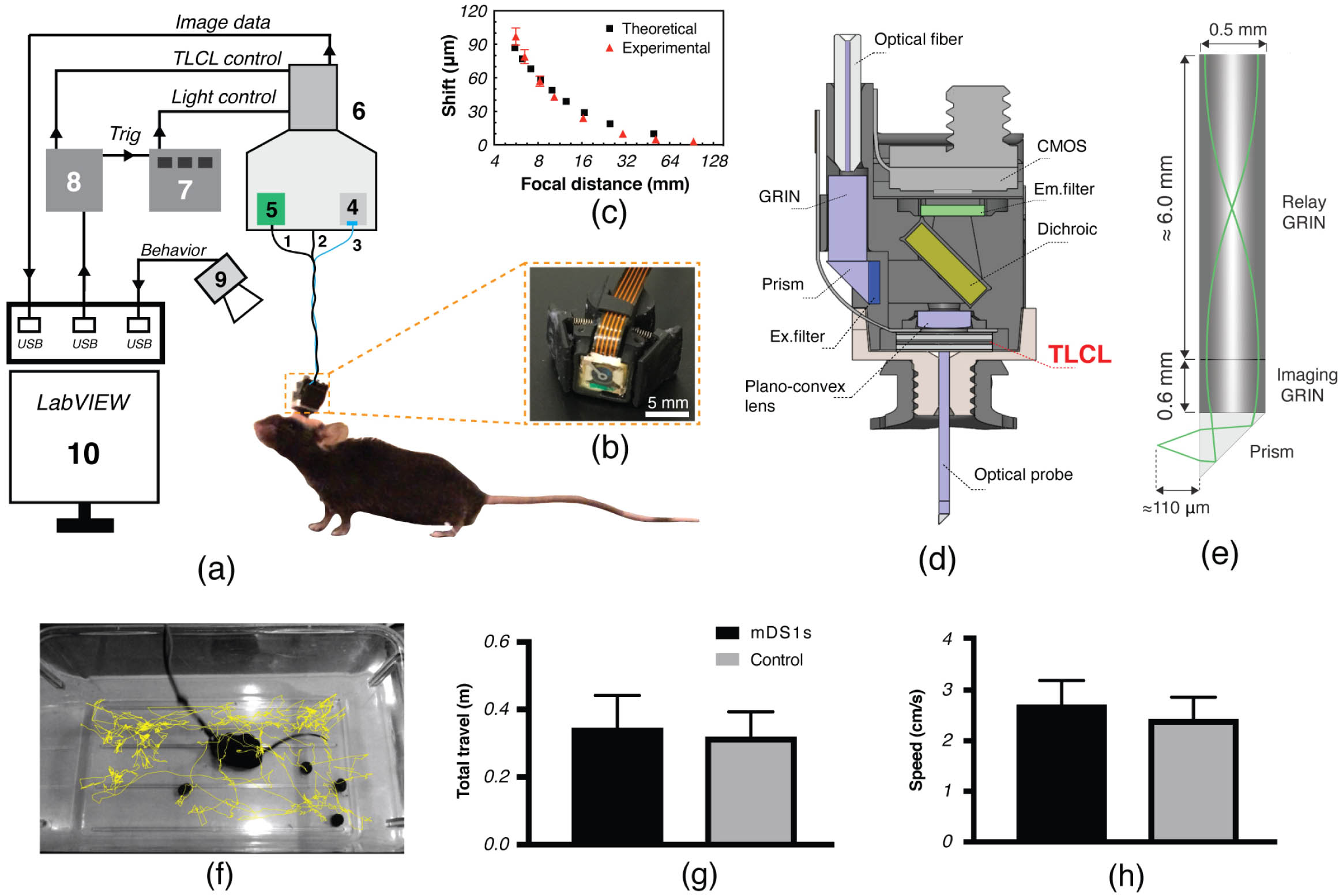
    Fig. 2. Schematic presentation of the ensemble of the imaging system. (a) Schematic of the system: 1, extension cable for the CMOS; 2, TLCL wires; 3, optical fiber; 4, light source; 5, DAQCMOS; 6, rotary joint system; 7, LED driver; 8, DAQLabVIEW; 9, camera to record behavior; and 10, LabVIEW user interface. (b) Photo of the TLCL within the mDS1s. (c) Electrically induced focal shift of the mDS1s simulated using Zemax optical software. Experimental results were obtained by measuring the FWHM of the point spread function of 1 μm diameter fluorescence. Error bars correspond to the standard deviation. (d) Schematic representation of optical components. Light from the optical fiber is first collimated by a large-diameter GRIN lens and then reflected by the 45° prism. The excitation filter is used to preserve the desired wavelengths and the dichroic mirror to reflect light into the plano-convex lens, toward the TLCL. Excitation light is then guided within the optical probe assembly to finally reach the object/structure of interest. The emission (fluorescent) light passes back through the probe to reach first the TLCL and then the plano-convex lens. The latter focuses the image on the CMOS sensor passing first through the dichroic mirror and the emission filter. (e) Schematic side view of the optical probe with three components: 45° prism, imaging (NA = 0.42), and rod GRIN (NA = 0.2) lenses. (f) Displacement path of the animal during the portability test (4  min). AnimalTracker plug-in (ImageJ) was used to track and analyze the animal’s movement. (g) Total traveled distance. (h) Average moving speed. Error bars correspond to the standard deviation.
    Electrical focal shift and characterization of optical parameters of the mDS1s. (a) Resolution and (b) magnification during electrical focal shift. Error bars correspond to standard deviations. (c) Scale bar samples imaged at different depths using the TLCL. Spacing between the lines is 10 μm. (d) In vitro depth imaging of GCaMP6 expressing neurons. The first row presents a sequence of images obtained with a miniaturized single-photon system (M1S) with a fixed imaging plane. The blur within the mechanically out-focused images (second and third columns) cannot be compensated. The second row presents a sequence of images obtained with our mDS1s. The electrical depth adjustment allowed us to refocus the images and to reveal the presence of neurons. The third row presents intensity normalization of the second row based on the fluorescence level of the central neuron (indicated by the red arrow). The thickness of the slice is 100±10 μm. (e) Intensity profile through the dotted line of interest in (d) (third row, lower-left corner) for the 80 μm focal shift. (f) The electrical scan shows various neuronal structures at different depths (indicated in the top left) within the in vitro slices presented in (a).
    Fig. 3. Electrical focal shift and characterization of optical parameters of the mDS1s. (a) Resolution and (b) magnification during electrical focal shift. Error bars correspond to standard deviations. (c) Scale bar samples imaged at different depths using the TLCL. Spacing between the lines is 10 μm. (d) In vitro depth imaging of GCaMP6 expressing neurons. The first row presents a sequence of images obtained with a miniaturized single-photon system (M1S) with a fixed imaging plane. The blur within the mechanically out-focused images (second and third columns) cannot be compensated. The second row presents a sequence of images obtained with our mDS1s. The electrical depth adjustment allowed us to refocus the images and to reveal the presence of neurons. The third row presents intensity normalization of the second row based on the fluorescence level of the central neuron (indicated by the red arrow). The thickness of the slice is 100±10  μm. (e) Intensity profile through the dotted line of interest in (d) (third row, lower-left corner) for the 80 μm focal shift. (f) The electrical scan shows various neuronal structures at different depths (indicated in the top left) within the in vitro slices presented in (a).
    Time-lapse imaging of Ca2+ activity from GCaMP6s-labeled neurons of the motor cortex. (a) Neuronal enhanced calcium activation image, (b) manually selected ROIs, (c) calcium traces, and (d) correlation map from the recorded neuronal activity (Visualization 1). Red to dark-blue colors represent maximal (1) and minimal correlation values (−0.6). (e) Structural reconstruction based on (d). Each dendritic branch (B) corresponds to multiple ROIs in (b); B1: 2, 3, 4; B2: 5, 6; B3: 7, 8; and B4: 24–29. (f) Neuronal activity was imaged and analyzed during three behaviors of the animal: resting, walking, and grooming. The treadmill was used to encourage walking comportment while, for the remaining conditions, the natural behavior of the animal was recorded. (g) Neuronal enhanced calcium activation image and (h) Ca2+ traces from somas (Sm) and dendrites (D) during the behavior in (f). Scale bar = 50 μm.
    Fig. 4. Time-lapse imaging of Ca2+ activity from GCaMP6s-labeled neurons of the motor cortex. (a) Neuronal enhanced calcium activation image, (b) manually selected ROIs, (c) calcium traces, and (d) correlation map from the recorded neuronal activity (Visualization 1). Red to dark-blue colors represent maximal (1) and minimal correlation values (−0.6). (e) Structural reconstruction based on (d). Each dendritic branch (B) corresponds to multiple ROIs in (b); B1: 2, 3, 4; B2: 5, 6; B3: 7, 8; and B4: 24–29. (f) Neuronal activity was imaged and analyzed during three behaviors of the animal: resting, walking, and grooming. The treadmill was used to encourage walking comportment while, for the remaining conditions, the natural behavior of the animal was recorded. (g) Neuronal enhanced calcium activation image and (h) Ca2+ traces from somas (Sm) and dendrites (D) during the behavior in (f). Scale bar = 50 μm.
    Electrical focus adjustment and time-lapse imaging of Ca2+ activity from GCaMP6s-labeled neuronal structures in the motor cortex of a freely behaving animal. (a) Images of neuronal activation at different, electrically adjusted focal depths. Focused structures are indicated with arrows (orange: soma, red: processes). Cropped images of (b) ROI 1 and (c) ROI 2, and (d) intensity profile through the dotted yellow line in (c). Scale bar = 5 μm. (e) Calcium activation images of the soma (Sm), dendrites (D), and spines (S) at two different depths: 0 μm and 60 μm (indicated on the top). Last column image was processed with the Lucy–Richardson deconvolution algorithm (itineration = 15) using DeconvolutionLab2 plug-in (ImageJ). (f) Intensity profile through the yellow line in (e). The diameter of S1 is ≈2.2 μm and the distance between S1 and D1 is ≈3.5 μm. (g) Enhanced calcium activation image (MIN1PIPE) with manually selected ROIs and (h) corresponding Ca2+ traces. Image plane was focused using the TLCL (60 μm). (i), (j) Head movement (j) of the animal was correlated (i) to the activity of electrically focused neuronal structures in (g).
    Fig. 5. Electrical focus adjustment and time-lapse imaging of Ca2+ activity from GCaMP6s-labeled neuronal structures in the motor cortex of a freely behaving animal. (a) Images of neuronal activation at different, electrically adjusted focal depths. Focused structures are indicated with arrows (orange: soma, red: processes). Cropped images of (b) ROI 1 and (c) ROI 2, and (d) intensity profile through the dotted yellow line in (c). Scale bar = 5 μm. (e) Calcium activation images of the soma (Sm), dendrites (D), and spines (S) at two different depths: 0 μm and 60 μm (indicated on the top). Last column image was processed with the Lucy–Richardson deconvolution algorithm (itineration = 15) using DeconvolutionLab2 plug-in (ImageJ). (f) Intensity profile through the yellow line in (e). The diameter of S1 is 2.2  μm and the distance between S1 and D1 is 3.5  μm. (g) Enhanced calcium activation image (MIN1PIPE) with manually selected ROIs and (h) corresponding Ca2+ traces. Image plane was focused using the TLCL (60 μm). (i), (j) Head movement (j) of the animal was correlated (i) to the activity of electrically focused neuronal structures in (g).
    Schematic demonstration of motionless focusing by reorientation of liquid crystal molecules (filled ellipses). (a) Different phase delays for different angles between the light wavevector k and the liquid crystal optical axis n; (b) uniform molecular orientation generates uniform phase delay; (c) non-uniform molecular orientation generates spherical phase delay and light focusing.
    Fig. 6. Schematic demonstration of motionless focusing by reorientation of liquid crystal molecules (filled ellipses). (a) Different phase delays for different angles between the light wavevector k and the liquid crystal optical axis n; (b) uniform molecular orientation generates uniform phase delay; (c) non-uniform molecular orientation generates spherical phase delay and light focusing.
    Characterization of the TLCL. (a) Optical power and (b) aberrations increase proportionally to the driven frequency of the AC square signal applied to the TLCL. The amplitude of the voltage varied from 2.4 V to 4.4 V. (c) RMS aberrations at the maximal optical power, for each optical power and driven voltage. The optimal voltage is 3.6 V; voltages below that value generated lower optical powers while having higher RMS errors.
    Fig. 7. Characterization of the TLCL. (a) Optical power and (b) aberrations increase proportionally to the driven frequency of the AC square signal applied to the TLCL. The amplitude of the voltage varied from 2.4 V to 4.4 V. (c) RMS aberrations at the maximal optical power, for each optical power and driven voltage. The optimal voltage is 3.6 V; voltages below that value generated lower optical powers while having higher RMS errors.
    Arutyun Bagramyan, Loïc Tabourin, Ali Rastqar, Narges Karimi, Frédéric Bretzner, Tigran Galstian. Focus-tunable microscope for imaging small neuronal processes in freely moving animals[J]. Photonics Research, 2021, 9(7): 1300
    Download Citation