
Yuan Chao, Peng Xu, Hanbing Tang, Fan Shi, Zhisheng Zhang. Illumination optimization method of LED light source for visual inspection system[J]. Infrared and Laser Engineering, 2021, 50(12): 20210745
- Infrared and Laser Engineering
- Vol. 50, Issue 12, 20210745 (2021)
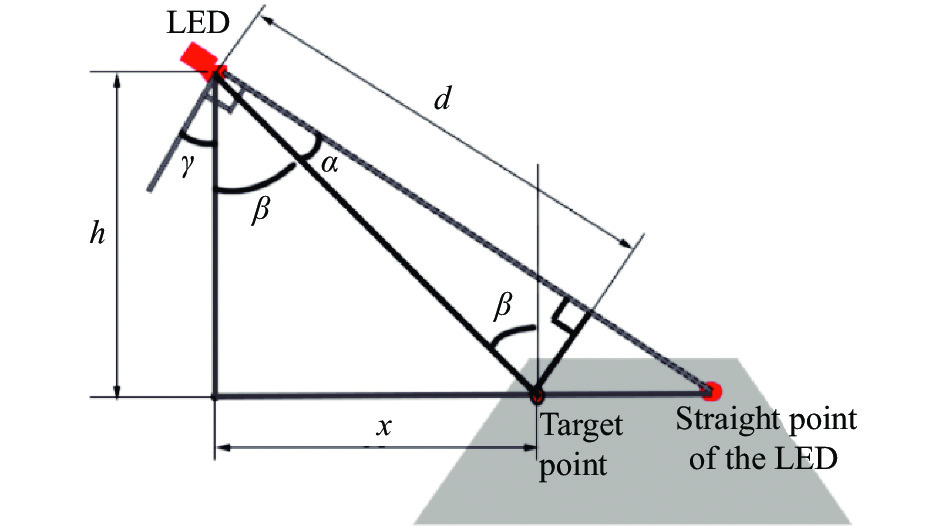
Fig. 1. Schematic diagram of single LED light source mathematical model
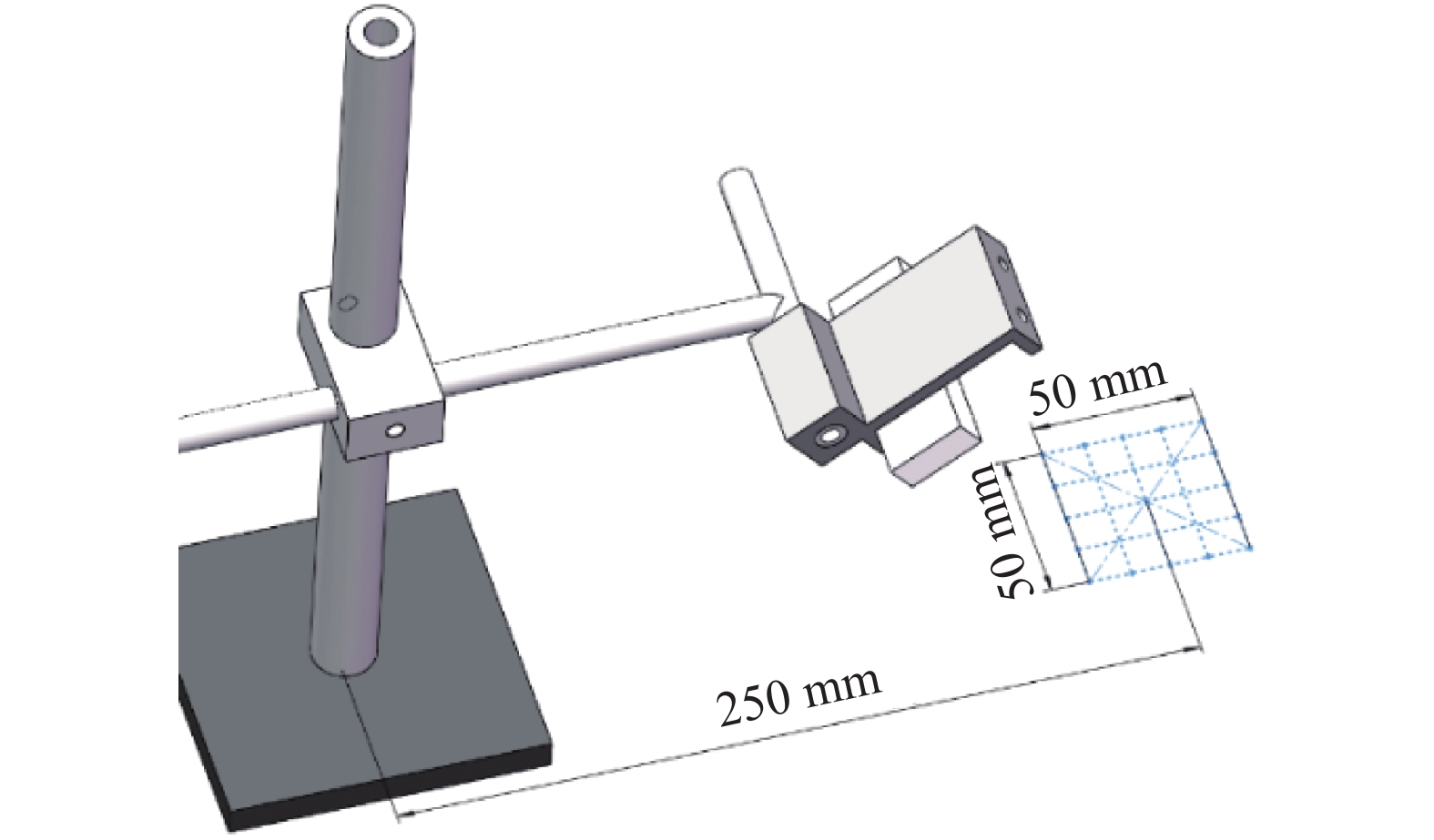
Fig. 2. Schematic diagram of the position of the measured plane
Fig. 3. Hardware environment of chip package quality inspection
Fig. 4. Schematic diagram of light source coordinate system
Fig. 5. Schematic diagrams of related parameters labeled in different coordinate systems
Fig. 6. Schematic diagram of vector analysis
Fig. 7. Flow chart of the original Salp swarm algorithm
Fig. 8. Convergence comparison of different algorithms
Fig. 9. Experimental platform of the plane illumination measurement
Fig. 10. Comparison of theoretical and actual relative illumination distribution
Fig. 11. Comparison of theoretical illumination of the measured plane and the background
Fig. 12. Illumination distribution along the X -axis when
changing by 1°
变化1°时X 轴方向上的照度分布
Fig. 13. Illumination distribution along the X -axis when
changing by 1°
变化1°时X 轴方向上的照度分布
Fig. 14. Illumination distribution along the X -axis when
changing by 10 mm
变化10 mm时X 轴方向上的照度分布
Fig. 15. Illumination distribution along the X -axis when
changing by 10 mm
变化10 mm时X 轴方向上的照度分布
Fig. 16. Comparison of optimization results and traditional forward illumination
|
Table 1. Initialization parameters of ISSA
|
Table 2. Evaluation function value corresponding to θ 1
|
Table 3. Evaluation function value corresponding to θ 2
|
Table 4. Evaluation function value corresponding to dx 2
|
Table 5. Evaluation function value corresponding to dz 2


Set citation alerts for the article
Please enter your email address

© Copyright 2018-2021 | Chinese Laser Press. All Rights Reserved 沪ICP备15018463号-20