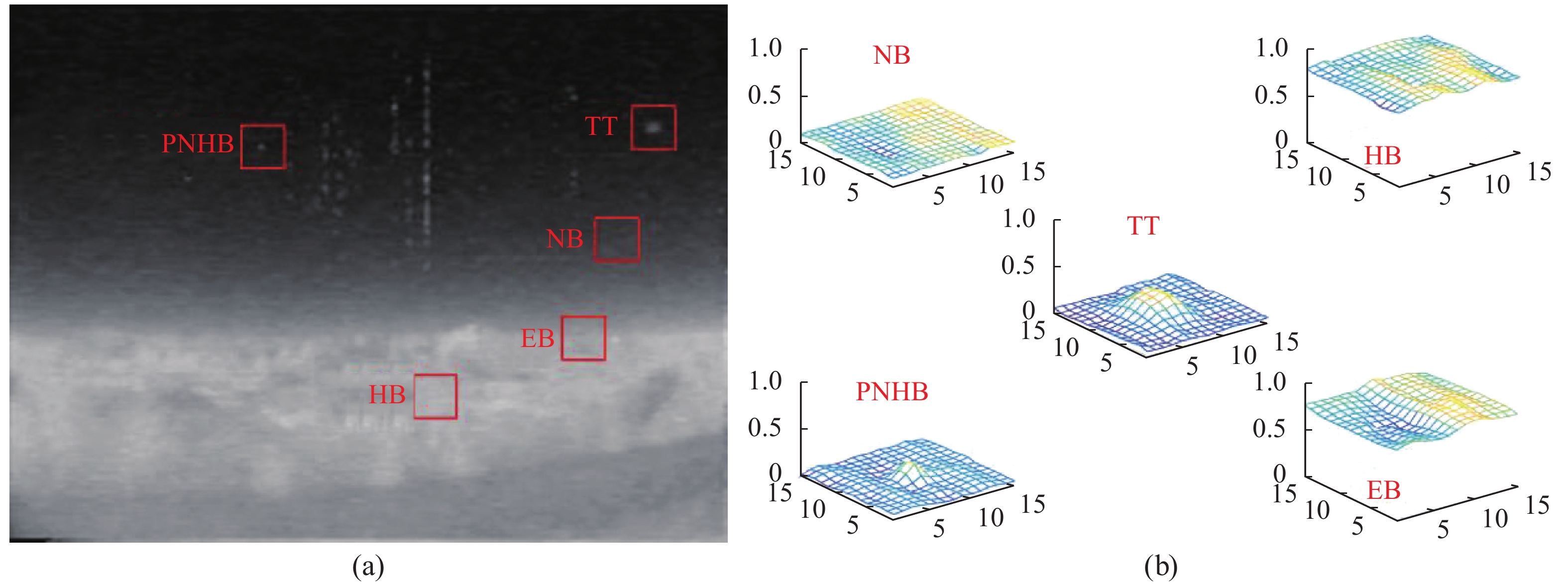
Fig. 1. (a) A sample of real IR image; (b) 3D distributions of different types of components. Here, TT represents true small target, NB represents normal background, HB represents high brightness background, EB represents complex background edge, and PNHB represents Pixel-sized Noises with High Brightness

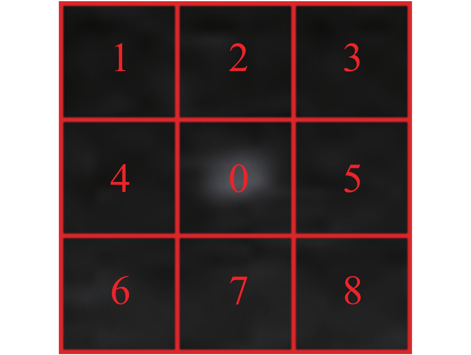
Fig. 2. A local small image patch used for MRDLCM calculation. It is divided into 9 cells, and the cell size N should be close to or slightly larger than real target

Fig. 3. Different cases when the central pixel of cell(0) is different

Fig. 4. Flow chart of the proposed algorithm

Fig. 5. Samples for the four IR sequences. (a) A sample for Seq. 1; (b) A sample for Seq. 2; (c) A sample for Seq. 3; (d) A sample for Seq. 4

Fig. 6. SCR results before and after MRDLCM calculation using different K for simulated data. (a) Target size is 3 × 3; (b) Target size is 5 × 5; (c) Target size is 7 × 7; (d) Target size is 9 × 9

Fig. 7. SCR results before and after MRDLCM calculation using different K for real sequences. (a) Seq. 1, target size is 7 × 5; (b) Seq. 2, target size is 5 × 5; (c) Seq. 3, target size is 3 × 3

Fig. 8. Calculation results for different types of pixels using the proposed MRDLCM_RLD algorithm. (a) Different cases when the central pixel of cell(0) is different; (b) The calculation result MRDLCM_RLD for the whole image using the proposed MRDLCM_RLD algorithm; (c) The 3D distributions of different types of components

Fig. 9. From top to bottom: the detection results using the proposed MRDLCM_RLD algorithm for Seq. 1, Seq. 2, Seq. 3 and Seq. 4. (a) The raw IR image samples of the four sequences; (b) The DFLCM result; (c)The RFLCM result; (d)The MRDLCM result; (e) The RLD result; (f) The MRDLCM_RLD result; (g) The threshold operation results, each connected area is regarded as a target

Fig. 10. Detection result using only MRDLCM alone for Seq. 3. (a) The raw IR image sample of Seq. 3; (b) The MRDLCM result; (c) The threshold operation result on MRDLCM, more false alarms emerge

Fig. 11. Comparisons of detection results between different algorithms, from top to down: the detection results of Seq. 1, Seq. 2, Seq. 3 and Seq. 4 using (a) DoG; (b) ILCM; (c) NLCM; (d) WLDM; (e) MPCM; and (f) RLCM

Fig. 12. ROC curves of different algorithms for (a) Seq. 1, (b) Seq. 2, (c) Seq. 3 and (d) Seq. 4

Table 1. Features of different sequences

Table 2. Characteristics of the first frame of the four sequences