
Yi Xu, Fu Li, Jianqiang Gu, Zhiwei Bi, Bing Cao, Quanlong Yang, Jiaguang Han, Qinghua Hu, Weili Zhang. Spectral transfer-learning-based metasurface design assisted by complex-valued deep neural network[J]. Advanced Photonics Nexus, 2024, 3(2): 026002
- Advanced Photonics Nexus
- Vol. 3, Issue 2, 026002 (2024)
Abstract
Keywords
1 Introduction
Compact 2D arrays consisting of subwavelength artificial meta-atoms, metasurfaces1 exhibit design flexibility for controlling electromagnetic (EM) waves, which has aroused widespread enthusiasm among researchers for multiple wavebands in optics and photonics. The intriguing advantages of metasurfaces enable versatile functionalities, such as focusing,2
However, the current deep-learning-based methods face the contradiction between efficiency and accuracy because they usually resort to a specific huge data set for reliable performance owing to their data-hungry nature. Collecting adequate data is slow and expensive, while training a DNN from scratch also involves considerable time consumption and computing resources. Once the feature space or distribution is changed, even though slightly different from the source task, the trained model may work ineffectively. To make the deep-learning-based methods more versatile for metasurface design, some solutions have been proposed to improve the model performance with a small data set. Transfer learning is a helpful framework that shares the knowledge and experience learned from the source model with the target one, so reduces the amount of required data and implements the prediction rapidly with high accuracy. In nanophotonics and metasurface design, transfer-learning-based methods are used to migrate knowledge between different physical scenarios, such as photonics films with different numbers of layers,32 and dielectric meta-atoms with different shapes or dimensions of cross sections. 33,34 Also the knowledge from other research fields can also be leveraged to study metasurfaces through transfer learning. For example, the meta-atoms are treated as images using the transfer-learning model based on GoogLeNet-Inception-V3 and realize the classification of phase from 0 to 360 deg.35 In addition to the transfer-learning-based method, data augmentation36 and spectral scalability37 were explored to reduce the dependence on data size, whereas previous works were limited to a fixed spectral range of the labeled data set. Once the range of the working waveband or the number of the sampling points changes, it is necessary to train a new model, and the training data set should be reprepared for this new task. Especially when material dispersion in different bands is considered, the scale invariance of Maxwell’s equations is no longer applicable. The method that exploits the spectral scalability by wavelength normalization trying to address this problem still suffers from a sudden deviation from the simulation data near the boundaries of the waveband range, which means the EM responses of the meta-atoms are not perfectly scalable.
In this work, we introduce a metasurface design methodology empowered by transfer learning that utilizes the commonality of the EM characteristics of the dielectric meta-atoms in different spectral ranges, thereby reducing the number of data by bridging the disparity of working frequencies. Specifically, we train the base model on an open-source data set25 in the infrared (IR) band from 30 to 60 THz and then store the knowledge gained in solving the source task, and transfer it to our terahertz (THz) spectral range from 0.5 to 1.0 THz to help the target task, which is trained on our small homemade data set. Here a complex-valued fully connected network that achieves high-performance spectral predicting ability is used in the source model, with an improvement of compared to the sum of its real-valued counterparts. We demonstrate three transfer strategies and experimentally quantify their performance, among which the “frozen-none” improves the prediction accuracy by compared to direct learning. Further, we propose several typical THz metadevices, including a metalens and a vortex beam generator, by employing the hybrid inverse model consolidating this trained target network and a global optimization algorithm as a proof-of-concept application. The simulated results clarify the reliability and scalability of our spectral transfer-learning-based metasurface design methodology assisted by complex DNN (CDNN), which is of great significance for balancing the efficiency and accuracy of the deep-learning-based method, hence promoting metasurface studies in arbitrary wavebands.
Sign up for Advanced Photonics Nexus TOC. Get the latest issue of Advanced Photonics Nexus delivered right to you!Sign up now
2 Results
2.1 Overall Framework of the Metasurface Design Methodology
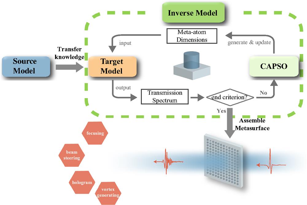
Figure 1 schematically illustrates the spectral transfer-learning-based metasurface comprehensive design framework, which consists of three primary submodules: (i) a deep-learning-based forward prediction source model trained on the massive open-source labeled data, (ii) a target model benefiting from the knowledge transferred from the source model then fine-tuned with a small homemade data set, and (iii) a hybrid inverse model for the on-demand metasurface design implemented by combining the trained target model with the conditioned adaptive particle swarm optimization (CAPSO) algorithm. The required transmission spectrum is fed into the inverse model as the design goal to retrieve the geometrical dimensions of the candidate meta-atoms, which are evaluated by comparing the predicted EM responses output from the well-trained target model and the desired goal. Then the optimization algorithm iteratively updates the generated dimensions until the maximum epoch or convergence criterion is reached. The efficacy of our proposed methodology is ultimately demonstrated by the performance of the metasurface assembled from the optimal meta-atoms at each position.
![]()
Figure 1.Flowchart of the spectral transfer-learning-based metasurface comprehensive design methodology assisted by the complex-valued DNN.
2.2 Source Spectral Model Construction
The source model is a data-driven feed-forward neural network, consisting of 11 fully connected layers that is aimed at dealing with the regression problem between the structure parameters and the EM responses of the meta-atoms. The fully connected network is capable of unveiling this implicit nonlinear relationship in a simplified and stable form, especially when the variables can be parameterized as tensors. Here the input and output parameters of the network as well as all the hyperparameters (weights and bias ) of each layer are extended to the complex domain to directly predict the complex transmission coefficients of meta-atoms, from which the phase and amplitude can be derived monolithically. In addition, the corresponding network functions, such as normalization, loss, nonlinear activation, and regularization functions, should also be adjusted to the form suitable for complex numbers. More detailed information about the CDNN has been included and discussed in Sec. 1 of the Supplementary Material. Using complex parameters has numerous advantages, including a richer and more versatile representation capacity and a more robust memory-retrieval mechanism, which has been demonstrated to improve the performance of the computer vision and audio-signal-processing tasks based on the CDNN compared to their real-valued counterparts.38 The architecture of CDNN is depicted in Fig. 2(a). The source-CDNN is first trained on the publicly released data set containing pairs of geometrical parameters and the real/imaginary parts of transmittance of the meta-atoms in the IR band. The input layer takes in a dimension tensor of size 4 including permittivity , radius , height , and the gap between adjacent meta-atoms, and the output tensor is the complex transmission coefficient sampled over 30 to 60 THz with an interval of 1 THz, giving a total of 31 elements. The supervised training process is conducted by minimizing the mean squared error (MSE) between the prediction result generated from the network and the ground truth given by full-wave simulations,
![]()
Figure 2.Schematic of the source model. (a) Illustration for the architecture and the parameters of the CDNN. (b) Learning curves of the CDNN that take the loss value as the function of the epoch. The smoothed train loss (blue curve) and test loss (red curve) are shown in the original learning curves (light gray). (c) Histogram of the MSE for the predicted complex transmission from the test set, where 95% of the data have an
In the total data set, a 70/30 split for the training and test data set is assigned. As the learning curve shown in Fig. 2(b), the overall test MSE is after 50,000 epochs. Figure 2(c) displays an MSE histogram of the predicted transmission from the test set, showing an average MSE of and a 95% data demarcation line , consistent with the low prediction error exhibited by the CDNN after training. Once the complex transmission coefficients are determined from the network, the corresponding phase and amplitude are calculated monolithically at each frequency, as shown in the right part of Fig. 2(a). Several samples are randomly selected from the test set as presented in Fig. S1 in the Supplementary Material, from which we can see that the network prediction results are in good agreement with the simulated truth values, even at those resonant frequency points, which demonstrates that CDNN has reasonably high predicting accuracy. To clarify the efficacy of the CDNN, we also trained two real-valued deep neural networks with real (RDNN) and imaginary (IDNN) parts as outputs, respectively. Detailed information on these two networks is described in Sec. 1 in Supplementary Material. The MSE of the CDNN is less than the sum of the MSE of the RDNN and IDNN, which are both after 50,000 epochs, indicating that the CDNN has superior performance compared with its real-valued counterparts. Given the vital role the source model plays in our transfer-learning-based method, such highly generalized predicting accuracy is critical to ensure the target model acquires sufficiently reliable knowledge to facilitate the on-demand metasurface design in the target task.
2.3 Transfer Knowledge to Target Spectral Model
Benefiting from the knowledge learned by the source model, the target model is trained on the target frequency domain (from 0.5 to 1.0 THz) to predict the complex transmission coefficients of the meta-atoms with a relatively small data set of 1000 samples. The relation of the interest bands of the source task and target task of spectral transfer learning is depicted in Fig. 3(a). The target data set of cylindrical-shaped all-dielectric meta-atoms is established via the commercial software CST Microwave Studio under -polarized normally incident light from 0.5 to 1.0 THz. In this home-built library, each meta-atom is determined by the same four geometry parameters as the above-mentioned ones in the open-source data set, but within a different range. The ranges of the four parameters are , , , and (all in ). The complex transmission coefficients over the whole spectrum are sampled into 51 frequency points with an interval of 0.01 THz. The simulation details are described in Sec. 1 in the Appendix. Then we employ transfer learning to help train the target neural network. The target model has the same network structure as the source model except for the output layer, whose dimensionality can be adjusted according to the sampling points of the target spectrum; in our case, there are 51 dimensions.
![]()
Figure 3.Schematic of transfer learning. (a) Diagram of the relation of interest bands of the source and target task and (b) illustration of spectral transfer learning. The top row is the architecture of the source model (blue), and the next rows are the target models (orange) based on three transfer strategies: frozen-none, copy-all, and hybrid-transfer, respectively. Blue blocks represent the copied layers from the trained source network and then are fine-tuned during training. Orange blocks represent the fine-tuned layers with random initialization. The mosaic pattern represents the frozen state. Black rounded rectangles represent activation layers.
We propose three transfer learning strategies as depicted in Fig. 3(b). (i) The target network copies the first layers from the source model as the initialization of weights and bias, and the remaining layers of the target network are randomly initialized with a normal distribution. The entire target network is fine-tuned simultaneously to be trained on the target data set and model, called the “frozen-none” strategy. (ii) The target network copies all hidden layers (except for the last one due to the mismatch of the dimensions) from the trained source model as the initialization of all hyperparameters. During the training process, the first layers are frozen, meaning that they do not change with training, and only the remaining layers are fine-tuned, called the “copy-all” strategy. (iii) The target network copies the first layers from the source model and freezes them, whereas the remaining layers are initialized and fine-tuned, called the “hybrid-transfer” strategy. Further details of the training setup (learning rates, etc.) are given in Sec. 2 of the Supplementary Material. As the major challenge in transfer learning is to select the general layers and specific layers to avoid the negative transfer between the source and target tasks, we conduct three sets of experiments to determine the best transfer-learning strategy as well as the most appropriate number of the transfer layers. The learning curves of these three strategies are shown in Fig. 4(a), and the colors from dark to light indicate the number of transfer layers from less to more, i.e., from 1(0) to 10(9). We aim not to maximize the absolute performance of the target model, but rather to verify that the transfer-learning-based method has advantages over direct learning. By comparing their performances on the same data set under consistent experimental conditions, we can see that in the frozen-none case, the test error is if trained from scratch, whereas it is around with the transferred knowledge, no matter how many layers are copied. The prediction accuracy is improved by about 26% through transfer learning. In addition, the loss function of transfer learning converges earlier than that of direct learning, manifesting a faster training speed. It takes an average of 72 min per 10,000 epochs of training on our computer equipped with an Nvidia RTX 3090 GPU, and our training process runs about 15,000 iterations to converge. In the other two cases, the test error is either higher or lower than that of direct learning as the number of transfer layers changes, which depends on the generality and specialization of different layers as well as the co-adaptation between neighboring layers.39 Our results show that the frozen-none strategy has stronger robustness than the other two, which can achieve higher accuracy than direct learning without careful parameter tuning, indicating it is more applicable for the spectral transfer target task.
![]()
Figure 4.Results of the spectral transfer learning. (a) Clusters of learning curves of three transfer strategies: frozen-none (red), copy-all (blue), and hybrid-transfer (orange). The colors from dark to light indicate the number of transfer layers from less to more. (b) Examples demonstrating the performance of the target CDNN using transfer learning.
Specifically, we use the frozen-none method of copying the first seven layers to train the target CDNN and test the generalization performance on the test set. Several typical test examples are presented in Fig. 4(b). These examples illustrate that the predicted spectra are in good accordance with the simulated ones in the regions, no matter whether the fluctuation is gentle or violent. It is also worth mentioning that this process only takes several milliseconds to calculate the transmission coefficients over the whole bandwidth under consideration of each meta-atom. Such prediction accuracy and efficiency are crucial for the on-demand metasurface design in the inverse model, as will be discussed in the next section.
2.4 Hybrid Inverse Model for the On-demand Metasurface Design
The core objective of the spectral transfer-learning-based method is the efficient and accurate on-demand metasurface design in the interested band. We divide the design task of the whole metasurface into the independent search for each meta-atom according to the phase and amplitude distribution oriented by functionality. In order to identify the optimal structure parameters at each pixel of the metasurface while avoiding the exponential growth of the simulation time during the iterations, we propose a hybrid inverse model that combines the data-driven deep-learning method with the rule-driven global optimization algorithm. In this model, the trained target-CDNN is regarded as an EM simulator to replace the traditional EM simulation software, which can precisely predict the transmission coefficients at an extremely high speed. The CAPSO algorithm performs to be a fast generator and a powerful optimizer of the meta-atoms. Specifically, the geometrical parameters given by CAPSO are fed into the target CDNN to predict the corresponding complex spectrum tensor, from which the extracted phases and amplitudes at certain frequencies are evaluated by quantifying the discrepancy between the current results and the goals. The optimal parameters are successively updated in iterative runs to reduce the value of the loss function [as Eq. (2) shows] until the maximum epoch is reached,
Instead of constructing an inverse or tandem DNN commonly used in the metasurface inverse design,29,40,41 we employ this hybrid model chiefly for these two reasons. (i) Previous inverse networks take the entire spectrum tensor as the input, which is suitable for the amplitude-functional devices in the continuous band, such as the filter, absorber, and resonators, whereas most phase-gradient metasurfaces only care about the EM responses at one or several frequencies, leaving the others alone. If the randomly assigned transmission is too different from the ones in the data set, the inverse network is almost impossible to output a reliable structure owing to nonuniqueness (a spectrum can be generated by multiple structural parameters, or no set of structural parameters can produce such a spectrum). (ii) The inverse model with the optimization algorithm can be readily modified to meet diverse design goals and restrictions.42 For example, we can impose a constraint in the equation on the parameter gap to alleviate the coupling among adjacent meta-atoms. We can also design frequency multiplexing devices with different numbers and values.
2.5 Metadevice Design and Verification
To verify the efficacy of our proposed hybrid inverse model, first we quickly design a focusing cylindrical metalens through this method. The ideal phase retardation provided by the metalens can be written as the function,
![]()
Figure 5.Characterization of the metalens designed by the hybrid inverse model. (a), (b) The target phase and amplitude profiles (blue lines) and the phases and amplitudes of the optimized meta-atoms at each pixel selected by our inverse model (red hollow circles). (c), (d) The theoretical and simulated normalized intensity distributions of the designed metalens along the propagation plane.
To further verify the efficiency and versatility of our method, we design a 2D metadevice for generating the focused THz vortex beam based on the function as follows:
![]()
Figure 6.Characterization of the metavortex generator designed by the hybrid inverse model. (a) The structure pattern, phase, and amplitude distributions of the designed metavortex generator output from the hybrid inverse model. (b), (c) The theoretical and simulated results for the phase, real part, and normalized intensity distributions along the
3 Discussion and Conclusions
We developed a spectral transfer-learning-based comprehensive methodology assisted by CDNN for the realization of the balance between computational efficiency and prediction accuracy to further help with the automated on-demand metasurface design in arbitrary wavebands. We explored the spectral transfer-learning strategy to ease the burden of large data volume requirements by migrating the learned knowledge from the original band to the target one by exploiting the commonality for EM properties of the all-dielectric meta-atoms with the same geometrical shape but in different spectral ranges. We proposed to utilize CDNN to train the source model on the given cheap data set, which obtains a fairly low prediction error of with an improvement of compared to its real-valued counterparts. We demonstrated that transfer learning can improve the prediction accuracy by in a quite short time compared to direct learning on the same small data set with only 1000 samples through the robust transfer-learning strategy named frozen-none. For proof of concept, we presented a focusing metalens and a metavortex generator working at 0.95 THz using the hybrid inverse model that combines the well-trained target CDNN with the CAPSO algorithm. The simulated results of these designed metadevice agreed well with the corresponding theoretical calculations, consequently validating the capability of the proposed comprehensive framework. In view of the underlying logic of our work, the deep-learning-based network is proposed to address the time and computing costs of the conventional simulation tools for metasurface design and modeling, i.e., our network aims at the numerical simulation process to demonstrate that the spectral transfer method is an efficient alternative to the consumed EM simulation software and human experience. As for the experiment demonstration, it will be the application of a well-trained feed-forward network. Our results show the potential to synchronously improve both the efficiency and accuracy of the deep-learning-based method, which will facilitate the fast and reliable metasurface design in arbitrary frequency bands, thus promoting the substantial application of deep learning in disciplines, such as meta-optics, spectral recognition, and resolution enhancement.
4 Appendix: Python-CST Co-Simulation
4.1 Random Generation of Meta-Atoms and Establishment of Data Sets
During the target data set establishment, the co-application of Python and CST automates the numerical simulations in a batched manner. The CST package provides a Python interface to the CST Studio Suite, which allows controlling a running simulation or reading the results of project files. First, we need to start a CST environment and create a new CST project. Then we edit the VBA codes to set up the model, materials, simulation conditions, and so on. Dimensions of the meta-atoms are randomly generated within their respective ranges, and they are constructed on top of a fused silica substrate with a thickness of and a fixed lattice size of . Each meta-atom is simulated under the -polarized plane wave by frequency domain solver with the tetrahedral mesh type. Periodic and perfectly matched layer (open) boundary conditions are used along the transverse ( and ) and longitudinal () directions with respect to the propagation of light. A field probe is placed at to detect the transmission spectrum of the meta-atom, which can be derived from the 1D results. One loop is completed for each simulation run, and the number of loops is the size of the target data set.
4.2 Arrange the Layout of Metasurfaces
During the verification process, the co-application of Python and CST automates the arrangement of the metasurface layout. Similarly, we start a CST project and initialize the settings. Then we input the dimension parameters of each meta-atom into CST and place them according to their corresponding positions through VBA codes to arrange them into a whole metasurface in order. The metadevice is simulated under an -polarized plane wave by a time-domain solver with a time duration of 500 ps. The boundary conditions in the propagation direction are set as open, and those in the and directions are set as open (for 2D metadevices, such as metalenses, vortex generators, and holographic plates) or period (for 1D metadevices, such as cylindrical metalenses and deflectors), as needed. Field monitors are placed according to the location of the electric field to be observed. Corresponding codes are provided by the authors.
Yi Xu received her BS degree in optoelectronic information science and engineering from Tianjin University, Tianjin, China, in 2019. Currently, she is working toward her PhD in optical engineering at the Center for Terahertz Waves, Tianjin University, Tianjin, China. Her research interests focus on dielectric metasurfaces, terahertz photonics, and machine learning for the design and optimization of metasurfaces.
Jianqiang Gu is a full professor at Tianjin University, China. He received his BEng degree in electronic science and technology, his MEng degree in physical electronics, and his PhD in opto-electronics technology from Tianjin University, China, in 2004, 2007, and 2010, respectively. Up to now, he has published more than 100 peer-reviewed journal papers with total citations of
Biographies of the other authors are not available.
References
[19] M. K. Chen et al. Artificial intelligence in meta-optics. Chem. Rev., 122, 15356-15413(2022).
[38] C. Trabelsi et al. Deep complex networks(2017).
[39] J. Yosinski et al. How transferable are features in deep neural networks?(2014).

Set citation alerts for the article
Please enter your email address
© Copyright 2018-2021 | Chinese Laser Press. All Rights Reserved 沪ICP备15018463号-20