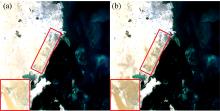
Fig. 1. Comparison of images before and after atmospheric correction
(a): Before atmospheric correction; (b): After atmospheric correction

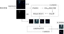
Fig. 2. Algorithm flow chart

Fig. 3. Spectral curves of typical surface features

Fig. 4. Comparison of NDWI and PNDWI extractions for seawater with and without sediment
(a): RGB image of seawater with sediment; (b): NIR image of seawater with sediment; (c): NDWI for seawater with sediment; (d): PNDWI for seawater with sediment; (e): RGB image of seawater without sediment; (f): NIR image of seawater without sediment; (g): NDWI for seawater without sediment; (h): PNDWI for seawater without sediment

Fig. 5. Statistical box plots of pixel values of 5 scenes in 4 bands and box plot interpretation
(a): Ship; (b): Thick clouds; (c): Thin clouds; (d): Smooth sea; (e): Sea clutter; (f): Box plot interpretation

Fig. 6. Process of assisting determination
(a): RGB; (b): NIR; (c): PNDWI; (d): Assisting determination

Fig. 7. An example of candidate region slice extraction

Fig. 8. (a)Schematic diagram of spectral feature extraction, (b)1×1 convolution diagram

Fig. 9. Channel shuffling diagram

Fig. 10. 1×1 Diagram of the LSGFNet network structure

Fig. 11. Part of the sample data for fine detection

Fig. 12. Loss reduction (a) and precision variation (b) of verification set with an interation of 10 000

Fig. 13. Detection result
(a): RGB; (b): NIR; (c): Binary images of rough detection; (d): Fine detection

Table 1. Rough dectection results of ships

Table 2. Comparison of lightweight network algorithms for test set

Table 3. Comparison of detection results by different algorithms