
Tianfu Li, Dexin Ba, Dengwang Zhou, Yuli Ren, Chao Chen, Hongying Zhang, Yongkang Dong. Recent progress in optical fiber sensing based on forward stimulated Brillouin scattering[J]. Opto-Electronic Engineering, 2022, 49(9): 220021
- Opto-Electronic Engineering
- Vol. 49, Issue 9, 220021 (2022)
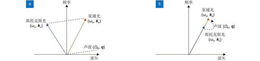
Fig. 1. Phase matching. (a) Backward stimulated Brillouin scattering; (b) Forward stimulated Brillouin scattering
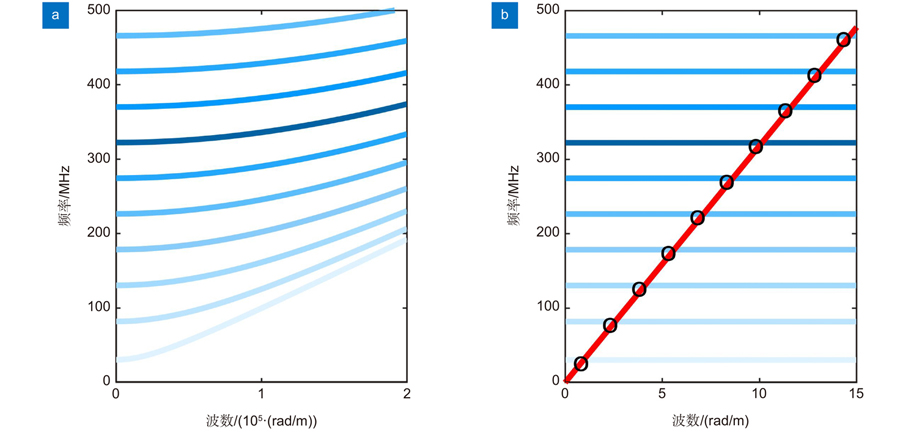
Fig. 2. Dispersion relation of R0,m-induced F-SBS. The bule solid lines represented the dispersion curve of acoustic waves, and the red one represented which of light wave. The shade of blue lines means the intensity of F-SBS.
Fig. 3. Transverse displacement profiles. (a) Radial mode R0,5; (b) Torsional-radial mode TR2,5
Fig. 4. Spectrum of R0,m modes induced F-SBS
Fig. 5. The schematic diagram of acoustic impedance sensing
Fig. 6. SI used to measure F-SBS
Fig. 7. The experimental set-up of F-SBS measurement based on SI. The excitation and probe light are separated by their different wavelengths[39]
Fig. 8. F-SBS in multi-core fiber. (a), (b) Transverse displacement profiles of modes R0,7 and R0,8; (c), (d) F-SBS spectrums measured in the inner core and outer core. The excitation light propagates in the inner core[43]
Fig. 9. F-SBS in polarization maintaining fiber. (a) Experimental set-up; (b) Measured F-SBS spectrums. The red trace is measured when the excitation light propagating in the fast axis, and probe in the slow axis; The black trace is measured in the opposite situation[41]
Fig. 10. F-SBS demodulation by LPG. (a) Schematic diagram; (b) Experimental set-up[45]
Fig. 11. Distributed F-SBS sensor based on local light phase recovery. The excitation and probe pulses are not only separated by wavelength, but also by time[36]
Fig. 12. Distributed F-SBS sensor based on local light phase recovery. (a) Distributed light intensity of 0, +1 and +2-order sidebands; (b) Phase accumulation along the fiber; (c) Distributed phase shift demodulated by differentiation; (d)~(f) Distributed F-SBS spectrums measured when the fiber under test placed in air, ethanol, and water[36]
Fig. 13. Principle of OMTDR. The energy transferred between the dual-frequency components of the pulses, and their Rayleigh scattering lights are used to demodulation[47]
Fig. 14. Distributed sensing results of OMTDR. (a)~(c) are the distributed F-SBS spectrums measured when the fiber under test placed in air, ethanol, and water[47]
Fig. 15. Schematic diagram of OMTDA[35]
Fig. 16. Schematic diagram of the fiber under test[48]
Fig. 17. Distributed results of OMTDA. (a) The energy transfer process along the fiber; (b) Distributed F-SBS gain spectrum[48]
Fig. 18. Results of acoustic impedance sensing. (a) The linewidth of spectrums along the fiber; (b) F-SBS spectrums measured in air and ethanol[48]
Fig. 19. Results of distributed diameter measurements[12]. (a) Diameter distribution before and after etching and its comparison with the SEM results (A-F); (b) Diameter variations along the FUT; (c) Representative images of the fiber cross section at A, B, C and E captured by SEM
Fig. 20. (a) Experimental setup for polarization separation assisted OMTDA; (b) Temporal trace and frequency components of activation and probing pulses[49]
|
Table 1. Acoustic impedance and F-SBS spectrum width of common substances


Set citation alerts for the article
Please enter your email address

© Copyright 2018-2021 | Chinese Laser Press. All Rights Reserved 沪ICP备15018463号-20