Fig. 1. NH zero mode in a three coupled cavities array: CMT model. (a) NH Hamiltonian. (b) Black symbols and lines: eigenvalues in the CMT model with τ0=0.2 and g=12.3 (inset: intensity and phase spatial distribution at M2 laser threshold). Red symbols and lines: eigenvalues in the CD-CMT model, for increasing carrier density N with a Gaussian profile N(x;x1)=exp[−(x−x1)2/σ2]N centered at cavity 1 (τc=7  ps, x1=60, σ=50, αH=2; other parameters can be found in Appendix A). (c) Logarithmic spectral intensity as a function of the center of a Gaussian pump spot, computed from Eq. (2) in the text. The pump spot profile is P(x;X)=exp[−(x−X)2/σ2], and γn(X)=P(xn;X), with σ=50 and γ=6, i.e., below laser threshold. Solid lines correspond to Re(εj) for j=1 (M1, blue), j=2 (M2, burgundy), and j=3 (M3, orange).

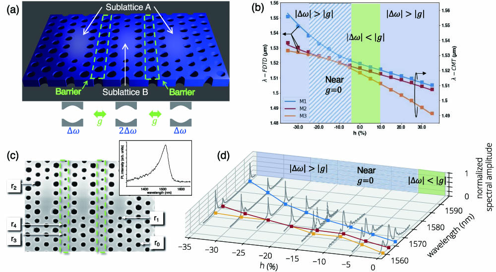
Fig. 2. Three coupled PhC cavities. (a) Artist view of the system, featuring controllable coupling by means of the two barriers (highlighted with dashed boxes) in which holes are modified. Two sublattices A and B can be defined, where couplings only take place between cavities belonging to different sublattices. Bottom: schematic representation showing how the presence of the barriers modifies the cavity detuning. The sublattice detuning is then Δω. (b) The 3D-FDTD simulation results of three coupled PhC cavities showing the evolution of the mode resonant wavelengths (symbols, left axis) as a function of the barrier parameter. Solid lines (right axis) are CMT predictions using polynomial approximations of g(h) and Δ(h) obtained from two coupled cavity FDTD simulations (see Appendix B). Two regions can be distinguished: the low (light green, |g|≳|Δω|) and high sublattice detuning regions (light blue, |g|<|Δω|); the near-zero coupling region is highlighted with a striped background. (c) SEM image of a sample of three coupled L3 InP-based PhC cavities. Inset: QW PL. (d) Normalized reflectivity spectra as a function of the barrier parameter from resonant scattering experiments. These results can be interpreted as the optical response of the coupled cavity system in the Hermitian limit.

Fig. 3. Spatially resolved PL measurements in the large detuning regime. (a) Experimental results showing spectral intensity maps upon spatial scanning of a pump spot for a=416  nm and h=−20%, Ppump=0.8  μW. The position of the sample is changed by means of the piezo-electric voltage. (b) CD-CMT predictions (σ=40, N=0.22, αH=3). Near-field [(a)-i to (a)-v, (b)-i to (b)-iii] and far-field [(a)-vi to (a)-x, (b)-iv to (b)-vi] images are displayed at the selected pump spot positions marked with horizontal dashed lines. Vertical white dashed lines in the near field indicate the position of the cavities, and kx=0 in the far field.

Fig. 4. Observation of the zero mode in the low detuning regime. (a) Experimental results showing spectral intensity maps upon spatial scanning of a pump spot for a=408 nm and h=0%, Ppump=0.8  μW. The position of the sample is changed by means of the piezo-electric voltage. (b) CD-CMT predictions (σ=40, N=0.27, αH=3). Near-field [(a)-i to (a)-iv, (b)-i to (b)-iii] and far-field [(a)-v to (a)-viii, (b)-iv to (b)-vi] images are displayed at the selected pump spot positions marked with horizontal dashed lines. Spectral filters are used in order to remove contributions from other modes, the spectral bandwidth being represented by the horizontal extension of dashed boxes. Vertical white dashed lines in the near field indicate the position of the cavities, and kx=0 in the far field.

Fig. 5. Two coupled PhC cavities’ 3D FDTD numerical simulations as a function of the barrier perturbation parameter h (see main text). (a) Hybrid mode frequencies. (b) Coupling and cavity detuning extracted from the hybrid mode frequency splitting and average, respectively. Solid lines are third-order polynomial fittings, which are subsequently used for CMT calculation with three coupled cavities in the main text.

Fig. 6. Single PhC cavity 3D FDTD numerical simulations in the presence of one or two barriers at the sides.

Fig. 7. Phase diagram underlying the transition from sublattice delocalization and zero modes to sublattice localization and mode coalescence. (a)–(e) Experimental PL intensity maps under pump spot position scanning across the coupled cavity system. (a)–(c) a=416  nm, Ppump=0.8  μW; (d), (e) a=408  nm, Ppump=1.1  μW. (f)–(j) CD-CMT and (k)–(o) linear CMT calculations with parameters αH=3, σ=40. (f)–(h) N=0.23, (i) N=0.24, and (j) N=0.27; (k)–(m) γ=1, (n) γ=1.1, and (o) γ=1.3.

Fig. 8. Zero-mode extinction due to full decoupling. (a) Experimental result on a sample with h=−20% featuring fabrication imperfections. A detuning of about 1 nm is observed between the extreme cavities. Notice that although three modes are observed around a pump position of 12 V, the three modes are localized into each cavity featuring different frequencies. The middle cavity is decoupled from the extreme one because of large negative h (localized phase). (b) CD-CMT simulations with h=−20%, N=0.225, αH=3, σ=40, and the cavity centered at x=140 is red-detuned by −6τ−1, equivalent to Δλ∼1.08  nm.

Table 1. Comparative Table with the Salient Properties of Hermitian and Non-Hermitian Photonic Zero Modes