
Zitong Xiong, Jian Ruan, Rongyu Li, Zhiming Zhang, Guangqiang He. Soliton formation with controllable frequency line spacing using dual pumps in a microresonator[J]. Chinese Optics Letters, 2016, 14(12): 121903
- Chinese Optics Letters
- Vol. 14, Issue 12, 121903 (2016)
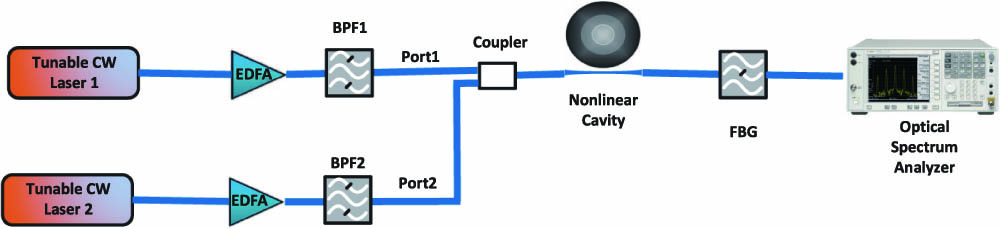
Fig. 1. Schematic illustration of the structure under study. Two CW pumps are amplified by an erbium-doped fiber amplifier (EDFA) and filtered by a bandpass filter (BPF) separately, then combined by a coupler with a ratio α 1 θ
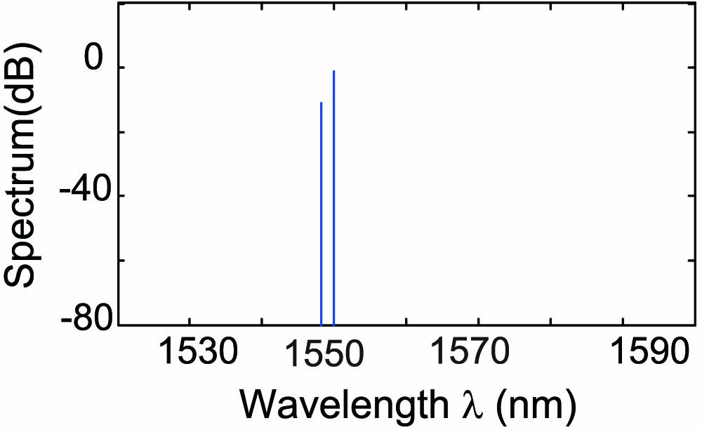
Fig. 2. Spectrum of the dual-pump field in the second step.
Fig. 3. (a), (b), and (c) show the evolution of the intracavity power and spectral and temporal profiles when scanning a laser over a monolithic Si 3 N 4 Q = 3 × 10 5 FSR = 226 GHz β 2 = − 4.711 × 10 − 26 s 2 m − 1 γ = 1 W − 1 m − 1 α = θ = 0.009 P in 1 = 0.755 W δ 0 = − 0.0045 L = 628 μm 4 × 10 − 3 ns − 1
Fig. 4. Same as Fig. 3 but with a slower tuning speed of 8 × 10 − 4 ns − 1
Fig. 5. (a) and (b) correspond to the temporal profile (left) and spectrum (right) of the intracavity field when pumped with a single CW pump at the end of the first step at simulation time t = 50 ns t = 625 ns
Fig. 6. Shows the route to the steady-state soliton of LLE. The left panel demonstrates the temporal evolution of intracavity field, where τ t t ≤ 50 ns
Fig. 7. (a) and (b) show the temporal profile and spectrum of the relationship between the steady-state solution in the second step and the total simulation time in the first step, respectively. (c) and (d) show the temporal profile and spectrum of a possible steady-state solution in the second step. (e) and (f) show the temporal profile and spectrum of another possible steady-state solution in the second step.
Fig. 8. Generated multi-FSR mode spacing solitons following the same steps and with the same resonator parameters used in Fig. 3 . (a), (b), and (c) correspond to f m = 2 FSR

Set citation alerts for the article
Please enter your email address
© Copyright 2018-2021 | Chinese Laser Press. All Rights Reserved 沪ICP备15018463号-20