An optical frequency comb (OFC) is a series of equidistant frequency lines that enables a variety of new applications in a wide range of topics that include precision spectroscopy, atomic clocks, ultracold gases, and molecular fingerprinting^[1]. OFC has been demonstrated both experimentally^[1,2] and theoretically^[3]. In theoretical models, coupled-mode equations^[3,4] and the Lugiato–Lefever model^[5] have been used to study the full spectral-temporal dynamics of parametric microresonator comb generation^[6–9]. Different coherence characteristics of different comb dynamical regimes have been identified^[10] and have obtained excellent agreement with past experiments.

It has been demonstrated that frequency combs can be converted into millimeter and terahertz regions through a photodiode and thus can be used as wireless communication spectral resources^[11]. To get a low-noise millimeter-wave source, soliton-state frequency combs are desired. Temporal solitons have excellent properties, such as broadband, low-noise frequency spectra, and small line-to-line amplitude variations^[12], and can maintain their shape in a temporal profile. They were first observed in fiber cavity in a 2010 experiment^[13]. Later, experimental observations of an oscillating Kerr cavity soliton (CS) and theoretical analyses of the one-dimensional CS dynamical instabilities in optical fiber resonators were performed^[14]. A sideband-controllable soliton mode-locked erbium-doped fiber laser has also been successfully demonstrated utilizing the nonlinear polarization rotation technique^[15]. In microresonators, temporal CSs have been experimentally observed by scanning through the cavity resonance^[16]. The number of solitons that circulate in the microresonator depends on the pump-laser detuning, while the temporal positions and how many CSs are excited have limited control^[10]. In contrast to fiber cavity experiments, the soliton pulses in microresonators form spontaneously, without the need for external stimulation. Besides scanning the pump-laser detuning, phase modulating the driving field has also been used to generate CSs in microresonators^[12,17]. Direct phase modulation of the cavity driving field has also been used in fiber cavities to selectively write and erase CSs at arbitrary positions^[18].

Controllable line-spacing frequency combs can be used as tunable millimeter-wave and terahertz sources. By launching two continuous-wave (CW) pumps at slightly different wavelengths into an optical fiber, tunable line-spacing frequency combs can be generated^[19]. It has also been demonstrated experimentally in an Si3N4 microring that controllable line spacing in the generated combs can be achieved by feedback and amplification at selected sidebands of an Si3N4 microring spectrum. By introducing a second input to an Si3N4 microring, stable twin solitons in a fiber cavity are formed^[20]. Multi-soliton states in a planar microresonator have been reached using soliton-induced Cherenkov radiation^[21]. The evolutions of cosine-modulated stationary fields relating to the generation of single-FSR or multi-FSR Kerr frequency combs in a microresonator were studied numerically^[22].

In this Letter, we propose another method for controllable frequency line-spacing soliton formation in microresonators by pumping the resonator with two CW pumps with a frequency spacing of multi-FSR. We start from the generalized Lugiato–Lefever equation (LLE) that describes the evolution of an intracavity field, and through numerical simulations, we find that only two steps are needed for soliton formation and only two fixed values of detuning are needed, thus solving the tuning speed problem. In addition, the method we propose has better control over the amount and location of the solitons traveling in the cavity compared to the tuning pump method. We also find that by introducing a second pump with frequency N FSR lower than the first pump at the proper time, multi-FSR solitons with N FSR comb spacing can be generated.

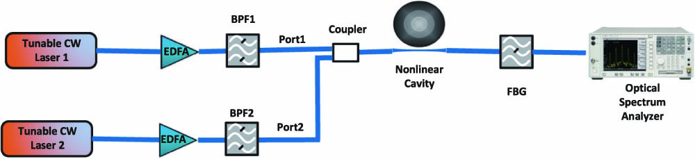
We consider the structure shown in Fig. 1. To study the evolution of the field inside the resonator, we use the mean-field LLE^[5,6] expressed by TR∂E(t,τ)∂t=(−α−iδ0+iLβ2k(i∂∂τ)2)E+iγL|E|2E+θEin′,(1)where E(t,τ) is the amplitude of the intracavity electric field, and t is the slow time describing the evolution of the field, while τ is the fast time describing the temporal field within the cavity in a frame. TR is the round-trip time of the field, and α, γ represent the total linear cavity losses and nonlinear coefficient, respectively. δ0 measures the frequency detuning between the laser carrier and cavity resonance frequencies. β2 is the second-order dispersion coefficient, which is also known as group velocity dispersion (GVD). Higher-order dispersion effects have been neglected. L is the cavity length, and Ein′ is the input field.

To simulate the dynamical evolution of an intracavity field, a split-step Fourier algorithm^[23] has been used. The parameters are taken from the 226 GHz FSR Si3N4 microresonator with a Q factor of 3×105 in Ref. [24]. The pump wavelength λp at 1550 nm from CW laser 1 is positioned in the anomalous GVD regime, for which β2=−47.11ps2/km. We start the numerical simulation from a weak initial Gaussian field, since the generated number of solitons generally varies when staring from a cold cavity^[10,12]. Two steps are taken in our simulation. In the first step, only a single CW pump with power Pin1=1.51W is coupled through port1 to excite frequency combs in the resonator. Pumping occurs at 1550 nm, the detuning δ0=0, and the input field in Eq. (1) can be expressed as Ein′=α1Pin1. After several ns, we have the second step: we set the detuning δ0=0.05 and introduce another CW pump fm away from the first laser with a pump power Pin2=0.151W through port2. Two fields are combined by a coupler with ratio α1=0.5 and coherently coupled into the resonator at the same time. Thus the dual-pump input field can be written as the following equation, Ein′=α1Pin1+(1−α1)Pin2exp(−2iπfmτ),(2)where Pin1 and Pin2 are the pump powers injected from port1 and port2, respectively, α1 is the ratio of the coupler, and fm describes the frequency spacing between the two pumps. Note that the frequencies of the two pumps are supposed to near different resonance frequencies. Figure 2 shows the spectral profile of the dual-pump input filed when the two pumps are separated by the FSR. We see two spectral lines in the spectrum. The spectral line with the lower amplitude corresponds to the pump from port2.

We first consider the conventional soliton formation method of blue-tuning the single pump laser^[16]. That is to say, a pump laser is scanned with a decreasing optical frequency ωp over a high-Q resonance. The scanning speed, also known as the tuning speed, is quite crucial in soliton formation. Figure 3 shows the evolution of the intracavity power and spectral and temporal profiles when scanning a laser over the resonance. The simulation parameters are taken from Ref. [24] and are listed in the caption. We can see that when the laser is tuning from the effectively blue-detuned regime through the effective zero-detuning frequency, the intracavity power increases slowly. At the same time, the spectrum begins to broaden, and the temporal profile begins to break into multiple pulses. When further tuning the laser into the effectively red-detuned regime, the intracavity power decreases and a single soliton forms. Then, we consider the situation of tuning the laser at a slower speed. Taking the same resonator parameters as Fig. 3, the simulation results are shown in Fig. 4. The evolution of the intracavity field is similar to that in Fig. 3, except multiple solitons form in the soliton regime. The simulation results further confirm that the single-pump tuning method indeed has limited control over the amount and location of the solitons traveling in the cavity^[10].

To have better control of the number and position of CSs, we propose the dual-pump method mentioned earlier. We first consider the situation of fm=FSR. Figure 5(a) shows the generated temporal and spectral profiles of the intracavity field at the end of the first step at simulation time t=50ns. It can be seen that the time domain profile consists of multiple pulses, and the spectrum is dominated by “primary” comb lines separated by multiple FSRs and a subharmonic higher-order comb^[3], which corresponds to the modulation instability (MI). The width of the temporal window is equivalent to the round-trip time of the field. Then we come to the second step, in which the resonator is pumped by two CW pumps separated by FSRs that are combined by a 50/50 coupler. At t=625ns (Fig. 5(b)), a single temporal CS forms, and the broadband frequency spectrum is quite smooth, with a comb mode spacing equivalent to the FSR. We can also see two peak spectral lines in the spectrum which correspond to the dual-pump input field. What needs to be pointed out is that we find a wide range of the second pump power is acceptable for soliton formation through our numerical simulation.

To make the route to a steady-state soliton more straightforward, we plot the temporal and spectral evolutions of the intracavity field from simulation time t=0 to 625 ns, as shown in Fig. 6. It can be seen that temporal pulses are generated from a cold cavity into nearly equidistant pulses in the first step, which corresponds to MI, and correspondingly, the spectral lines arise and broaden due to cascaded four-wave mixing (FWM). From the presence of another pump at t=50ns in the second step, the number of pulses decreases suddenly into random pulses, and the spectrum clearly broadens. The number of pulses continues to decrease in the coming period of time, and the spectrum exhibits periodic broad fluctuations, which eventually leads to the generation of a single-CS with a broadband and smooth spectrum. What needs to be pointed out is the value of cavity detuning that we choose for each step. In the first step, we set δ0=0, which means the pump frequency is equivalent to the resonance frequency. This step is similar to the beginning, when we generated solitons through the effective blue-detuned operation^[8,16]. Thus, the generated field corresponds to the characteristics of the MI^[10]. Another pump is introduced in the next step. It has been demonstrated previously in experiments that the laser frequency needs to be tuned through effective zero detuning^[16]. Then, we change the value of the pump detuning δ0 to 0.05. This value is in the stable-CS region of the blue-detuned approach^[8]. It has also been demonstrated that the tuning speed is quite crucial in the sweeping pump-resonance detuning method^[16]. Thus, in comparison, the method we propose is much simpler, since only two fixed detuning points are needed, thus bypassing the tuning speed problem.

Then we consider the situation of changing fm to 4 FSR. Using the same resonator parameters as in Fig. 3, we still pump the resonator with a single pump through port1 with Pin1=1.51W and δ0=0. After several ns, we change δ0 to 0.05 and introduce another pump with Pin2=0.151W, with frequency 4 FSR higher than that of the first pump. Through the simulation, we find that the generated amount and location of the steady-state solitons in the second step have a close relationship with the simulation time of the first step. The results are shown in Fig. 7. The Y labels in Figs. 7(a) and 7(b) stand for the total simulation times of the first step, ranging from 15 to 75 ns. We can see that the first step simulation time affects the steady-state solution of the second step to some extent. There exist two kinds of soliton states. The steady state shown in Figs. 7(c) and 7(d) has four solitons that are equidistance within one round trip, and the spectrum is broad and smooth, with 4 FSR mode spacing. The steady state shown in Fig. 7(e) has three solitons within one round trip, and its temporal profile is similar to the profile when one of the four solitons within a round trip is absent from the first state. The latter steady-state spectrum shown in Fig. 7(f) is interesting because despite the fact that the spectrum has single FSR mode spacing, the spectral lines with multiple 4 FSR away from the pump are enhanced. These two kinds of steady state spectra observed in Fig. 7 can be understood by considering the interactions between the dual-pump fields. The introduction of another pump in the second step can be seen as a way of modulating the intracavity field. Thus, the spectral lines with multiple fm away from the pump are enhanced. We can explain the relationship between the final steady state and the first step time by considering the comb instability at the first step. The comb instability feature in the first step determines the uncertainty of the mode phase relationship, eventually leading to different kinds of mode competition in the second step. As a result, different soliton states form in the second step. Compared to the single-pump laser tuning method, the method we propose has better control over the amount and location of the solitons traveling in the cavity.

We consider the situation of changing fm to multi-FSR. Using the same resonator parameters as in Fig. 3, we still pump the resonator with a single pump through port1 with Pin1=1.51W and δ0=0. After several ns, we change δ0 to 0.05 and introduce another pump with Pin2=0.151W, with frequency N FSR higher than the first pump. The generated temporal profile and spectrum of the steady state intracavity field are shown in Fig. 8. Figures 8(a)–8(c) correspond to 2FSR, 3FSR, and 4FSR spacing of the dual pump, respectively. We can see from the results that fm has a close relationship with the generated soliton number. Assuming fm to be equivalent to N FSR, then we can get N solitons that are equidistant per round trip in the temporal profile, and correspondingly, a smooth spectrum with mode spacing equivalent to N FSR forms in the spectrum. We note that the simulation time of the first step has a close relationship with the generated soliton: neither too short nor too long of a simulation time in the first step will lead to the generation of multi-FSR mode spacing solitons, which we have discussed. However, after some trial and error, it is easy to find the most suitable time for the first step to generate multi-FSR mode spacing solitons. Thus, multi-FSR solitons can be generated by changing the spacing between two pumps.

In conclusion, we propose a new approach to the formation of controllable frequency line-spacing solitons and numerically study the evolution of the intracavity field using LLE. The demonstrated technique offers a simpler way of generating solitons compared to the scanning detuning method, since there is no tuning speed problem. In addition, the method we propose has better control over the amount and location of the solitons traveling in the cavity compared to the tuning pump method. We also find that by introducing a second pump with frequency N FSR lower than the first pump at proper time, multi-FSR solitons with N FSR comb spacing can be generated.