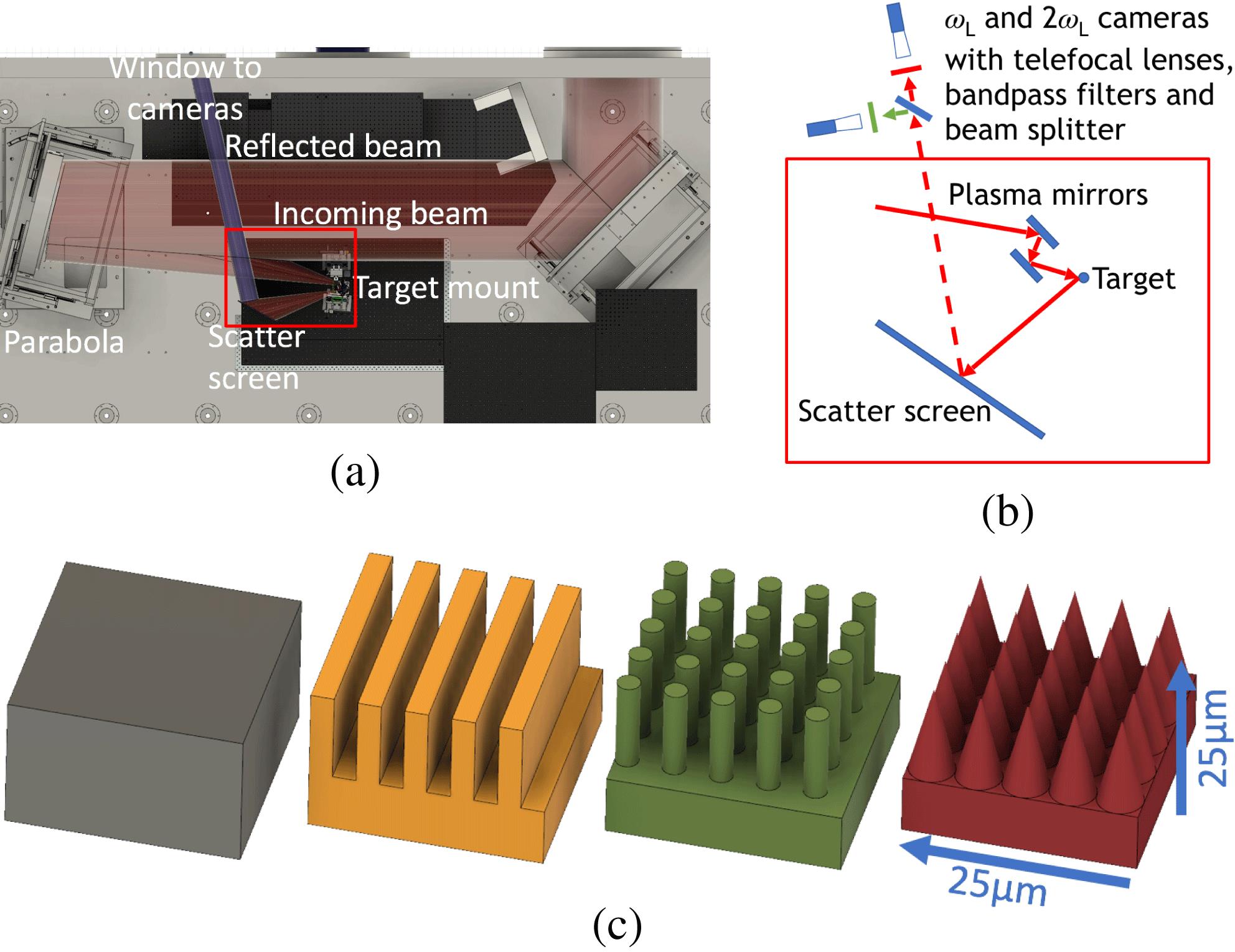
Fig. 1. (a) Plan view of the experiment arrangement inside the vacuum chamber. The incoming laser beam is shown in red and light reflected out of chamber to the CCDs is shown in blue. (b) Schematic showing the path of the incoming laser beam (solid red line), from the double plasma mirror onto target and finally onto the scatter screen. The imaging line is shown by the dashed red line. (c) Schematic illustrating the four types of targets employed; from left to right: flat foil, grooves, pillars and needles.

Fig. 2. Measurements of the spatial-intensity distribution of the laser light reflected from the plasma critical density surface, at fundamental and second harmonic frequencies, as captured on a scatter screen, with dashed red line denoting the expected specular direction. Images (a) and (b) correspond to the $\unicode[STIX]{x1D714}_{L}$ and $2\unicode[STIX]{x1D714}_{L}$ signals for the flat foil target, respectively. (c) and (d) are the same for the groove target, (e) and (f) are for the pillar target, and (g) and (h) are obtained with the needle target. The scale presented in (a) and (b) is the same for all $\unicode[STIX]{x1D714}_{L}$ and $2\unicode[STIX]{x1D714}_{L}$ images, respectively.

Fig. 3. Normalized line-outs from the measured (a) $\unicode[STIX]{x1D714}_{L}$ and (b) $2\unicode[STIX]{x1D714}_{L}$ reflected light patterns produced by the groove target. The dashed lines correspond to the expected positions of light maxima from diffraction theory.

Fig. 4. PIC simulation results showing electron density (and thus the groove expansion) for a laser intensity of $5\times 10^{19}~\text{W}\cdot \text{cm}^{-2}$, pulse duration of 500 fs (FWHM) and $7~\unicode[STIX]{x03BC}\text{m}$ focal spot (FWHM), for (a) $t=-500~\text{fs}$ and (b) $t=0$. Overdense plasma is shown in red while underdense plasma is shown in blue. The green line in (b) shows the critical density trace as used in the ray-tracing model.

Fig. 5. Contour plot showing the evolution of the target profile (the plasma critical density surface) as determined from modelling the plasma thermal expansion.

Fig. 6. (a) Magnified view of the top of three groove structures showing reflected light rays, for light incident vertically downwards. (b) Separation of light maxima at the distance of the scatter screen as a function of the groove depth, as determined from the ray-tracing model.

Fig. 7. (a) Groove depth as a function of electron temperature, as determined from the numerical thermal expansion model. (b) Plot of results from numerical modelling, showing expected separation between maxima in reflected light (at the distance of the scatter screen) as a function of plasma electron temperature. The red line represents the numerical model and black dots are data points from the PIC simulations.

Fig. 8. Intensity distribution determined from a Huygens–Fresnel model at a plane 1 mm from an evolved groove structure as a function of $A$, with $S=5~\unicode[STIX]{x03BC}\text{m}$ and laser focal spot FWHM equal to (a) $2~\unicode[STIX]{x03BC}\text{m}$ and (b) $7~\unicode[STIX]{x03BC}\text{m}$. The solid lines indicate the expected first order diffraction position and the dashed lines correspond to the results determined from the model.

Fig. 9. Intensity distribution determined from a Huygens–Fresnel model at a plane 1 mm from an evolved groove structure as a function of $S$, with $A=4~\unicode[STIX]{x03BC}\text{m}$ and laser focal spot FWHM equal to $7~\unicode[STIX]{x03BC}\text{m}$. (b)–(d) The intensity profile as the phase of the structure is varied for (b) $S=35~\unicode[STIX]{x03BC}\text{m}$, (c) $S=20~\unicode[STIX]{x03BC}\text{m}$ and (d) $S=5~\unicode[STIX]{x03BC}\text{m}$.