• Chinese Optics Letters
  • Vol. 15, Issue 3, 030013 (2017)
F. Wackenhut1, B. Zobiak2, A. J. Meixner1, and A. V. Failla1、2、*
Author Affiliations
  • 1Eberhard Karls University Tübingen, Institute of Physical and Theoretical Chemistry, Tübingen 72076, Germany
  • 2University Medical Center Hamburg-Eppendorf, UKE Microscopy Imaging Facility, Hamburg 20246, Germany
  • show less
    DOI: 10.3788/COL201715.030013 Cite this Article Set citation alerts
    F. Wackenhut, B. Zobiak, A. J. Meixner, A. V. Failla. Tuning the fields focused by a high NA lens using spirally polarized beams (Invited Paper)[J]. Chinese Optics Letters, 2017, 15(3): 030013 Copy Citation Text show less
    Passing through two MCs, a linearly polarized Gaussian beam is turned into an SPDB. MC1 is used to produce an RPDB. MC1 is composed of an LQMC and a spatial filter produced by two confocal lenses (L1/2) with a properly sized pinhole (PH) in between. MC2 turns an RPDB into an SPDB by employing two λ/2 retardation wave plates (WP1/2), one fixed and the other variable in order to change the angle β.
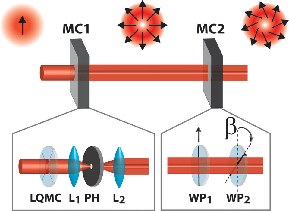
    Fig. 1. Passing through two MCs, a linearly polarized Gaussian beam is turned into an SPDB. MC1 is used to produce an RPDB. MC1 is composed of an LQMC and a spatial filter produced by two confocal lenses (L1/2) with a properly sized pinhole (PH) in between. MC2 turns an RPDB into an SPDB by employing two λ/2 retardation wave plates (WP1/2), one fixed and the other variable in order to change the angle β.
    Intensity distribution visualization of relevant SPDBs produced using λex=633 nm and by focusing the light with an NA=1.25 oil objective lens. First row: intensity profile of the longitudinal component (red continuous line) and the transversal component (blue dashed line). Second row: simulated images of relevant SPDBs. Third row: corresponding value of γ. The following beams have been considered: (a) and (f) RPDB; (b) and (g) SPDB with longitudinal and transversal field components set to be the same; (c) and (h) SPDB with S/P polarized component set to be the same; (d) and (i) SPDB characterized by |Ex|max⁡=|Ey|max⁡=|Ez|max⁡; (e) and (j) APDB.
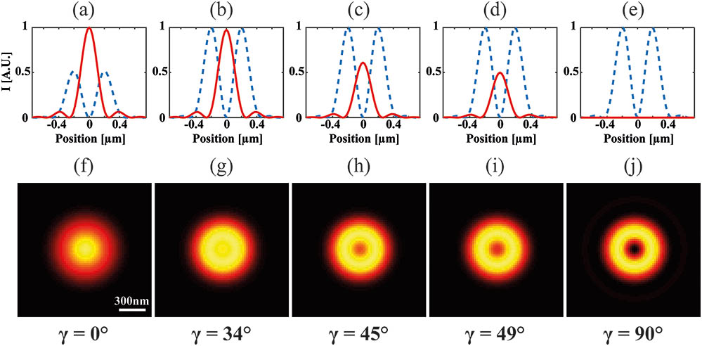
    Fig. 2. Intensity distribution visualization of relevant SPDBs produced using λex=633nm and by focusing the light with an NA=1.25 oil objective lens. First row: intensity profile of the longitudinal component (red continuous line) and the transversal component (blue dashed line). Second row: simulated images of relevant SPDBs. Third row: corresponding value of γ. The following beams have been considered: (a) and (f) RPDB; (b) and (g) SPDB with longitudinal and transversal field components set to be the same; (c) and (h) SPDB with S/P polarized component set to be the same; (d) and (i) SPDB characterized by |Ex|max=|Ey|max=|Ez|max; (e) and (j) APDB.
    In plane polarization rotation α of a focused SPDB versus in plane polarization rotation γ of a collimated SPDB (red circled line). The beam is focused by an objective lens of the (a) NA=1.25 or (b) NA=1.45. In both cases, γ is plotted versus γ (blue squared lines) to emphasize the differences between α and γ. The ratio between SPDB transversal and longitudinal field intensity after focusing with a lens with the (c) NA=1.25 or (d) NA=1.45, plotted as a function of the angle α (red continuous line) and γ (blue dashed line).
    Fig. 3. In plane polarization rotation α of a focused SPDB versus in plane polarization rotation γ of a collimated SPDB (red circled line). The beam is focused by an objective lens of the (a) NA=1.25 or (b) NA=1.45. In both cases, γ is plotted versus γ (blue squared lines) to emphasize the differences between α and γ. The ratio between SPDB transversal and longitudinal field intensity after focusing with a lens with the (c) NA=1.25 or (d) NA=1.45, plotted as a function of the angle α (red continuous line) and γ (blue dashed line).
    2D/3D orientational visualization of a gold nanorod’s one photon luminescence patterns excited by SPDBs. First row: schematic drawings of the collimated SPDBs used for excitation. Second row: one photon luminescence patterns of the same individual gold nanorod excited by the SPDBs schematically depicted in the first row. Third row: simulated one photon luminescence patterns of a single gold nanorod excited by the SPDBs depicted in the first row. Fourth row: shows the values of γ (roughly estimated by rotating the λ/2 retardation wave plate), αt (determined from the theoretical patterns), and αs (estimated from the experimental patterns). Fifth and sixth rows: visualization of the experimentally determined (fifth) and the theoretically generated (sixth) one photon luminescence pattern of the same gold nanorod excited by the SPDBs that are schematically shown in the first row.
    Fig. 4. 2D/3D orientational visualization of a gold nanorod’s one photon luminescence patterns excited by SPDBs. First row: schematic drawings of the collimated SPDBs used for excitation. Second row: one photon luminescence patterns of the same individual gold nanorod excited by the SPDBs schematically depicted in the first row. Third row: simulated one photon luminescence patterns of a single gold nanorod excited by the SPDBs depicted in the first row. Fourth row: shows the values of γ (roughly estimated by rotating the λ/2 retardation wave plate), αt (determined from the theoretical patterns), and αs (estimated from the experimental patterns). Fifth and sixth rows: visualization of the experimentally determined (fifth) and the theoretically generated (sixth) one photon luminescence pattern of the same gold nanorod excited by the SPDBs that are schematically shown in the first row.
    F. Wackenhut, B. Zobiak, A. J. Meixner, A. V. Failla. Tuning the fields focused by a high NA lens using spirally polarized beams (Invited Paper)[J]. Chinese Optics Letters, 2017, 15(3): 030013
    Download Citation