Tuning the fields focused by a high NA lens using spirally polarized beams (Invited Paper)

F. Wackenhut; B. Zobiak; A. J. Meixner; A. V. Failla

doi:10.3788/COL201715.030013

Abstract

We show the power of spirally polarized doughnut beams as a tool for tuning the field distribution in the focus of a high numerical aperture (NA) lens. Different and relevant states of polarization as well as field distributions can be created by the simple turning of a

λ / 2

retardation wave plate placed in the excitation path of a microscope. The realization of such a versatile excitation source can provide an essential tool for nanotechnology investigations and biomedical experiments.

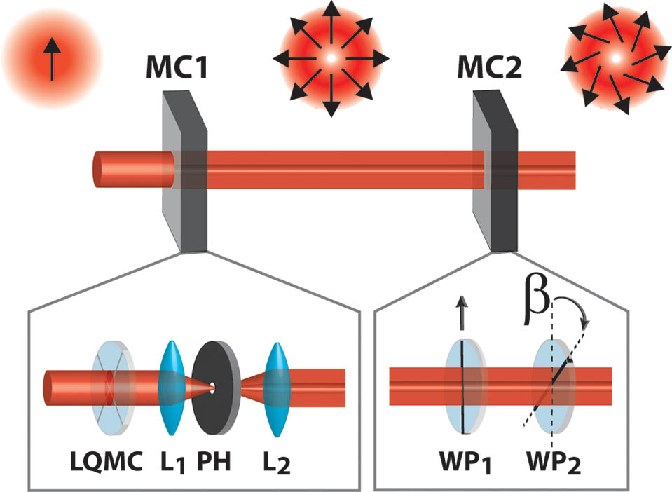
In the last two decades, enormous progress has been achieved in the fields of light microscopy, nanoscopy, and, in more general terms, nanotechnology. Super-resolution, far-, and near-field microscopy made the visualization of nano-objects possible with an optical resolution of about 10 nm. These revolutionary improvements allowed researchers to make important steps forward in many fields, e.g., nanotechnology and biology, see Refs. [1,2]. In parallel, the exploitation of anisotropic polarized excitation sources like radially/azimuthally polarized doughnut beams (R/APDBs) have been essential, e.g., for increasing the excitation and detection efficiency in near-field tip-enhanced microscopy^[3,4], revealing the orientation, shape, and structure of strongly polarized nanostructures^[5–8], or increasing the ability to disclose the organization of collagen domains in animal and human skin^[9]. These and other prominent studies have relied on sophisticated and ingeniously made light sources integrated into self-build microscopes. In many cases, a single and unique device was designed for only one special application. In the present days, however, the standardization and integration in easily accessible and flexible setups of highly sophisticated imaging approaches is a necessary prerequisite for further scientific progress. Especially for the development of bio-oriented nanotechnologies, microscopes are required to be provided with multiple and tuneable light sources. In this Letter, we show how a source of variable spirally polarized doughnut beams (SPDBs) can fulfill these requirements. SPDBs form a family of anisotropically polarized fields, i.e., the polarization varies point by point, but is linear at any individual point. Relevantly, RPDBs/APDBs are special cases of SPDBs^[10,11]. A practical way to realize SPDBs is presented in Fig. 1. It makes use of two mode converters (MCs). First, an RPDB is realized using a liquid crystal MC (LQMC) according to the procedure described in Ref. [12]. Second, the polarization of the RPDB is uniformly rotated by angle $β$ using a series of two $λ / 2$ retardation wave plates, where one is fixed while the other is free to rotate^[13]. Please note that the rotation of the second $λ / 2$ retardation wave plate (labeled as WP2 in Fig. 1) permits to change $β$ .

Figure 1.Passing through two MCs, a linearly polarized Gaussian beam is turned into an SPDB. MC1 is used to produce an RPDB. MC1 is composed of an LQMC and a spatial filter produced by two confocal lenses ( $L_{1 / 2}$ ) with a properly sized pinhole (PH) in between. MC2 turns an RPDB into an SPDB by employing two $λ / 2$ retardation wave plates ( ${WP}_{1 / 2}$ ), one fixed and the other variable in order to change the angle $β$ .

Since the RPDBs and APDBs are an orthogonal set of beams, they can be used to describe the field $E_{SPDB}$ of a generic SPDB in the following way: $E_{SPDB} = E_{APDB} \sin γ + E_{RPDB} \cos γ,$ (1)where $γ = 2 β$ (with respect to Fig. 1) is a fixed rotation angle, and $E_{(RPDB / APDB)}$ is the field distribution of an RPDB/APDB. It is straightforward that RPDBs are generated by setting $γ = 0 °$ , while the original RPDB is converted into an APDB by setting $γ = 90 °$ . As mentioned before, different light microscopy applications need different excitation sources, but more precisely they require different conformations of the field distribution in the focus of a high numerical aperture (NA) lens. For example, in some experiments it is crucial to control the ratio between the senkrecht/parallel (S/P) polarized components of the focused field^[14]. In other cases, see for example Ref. [15], it is important to tune the ratio between the field polarized along the optical axis, i.e., the longitudinal field, and the field polarized along the focusing plane, i.e., the transversal field. Moreover, precise control of the field distribution in the focus can be beneficial for applications like second-harmonic generation (SHG) microscopy^[9], where it can be useful to adjust and control the relative strength of the field along all directions and, as a special case, to realize a polarization state, where $| E_{x} |_{\max} = | E_{y} |_{\max} = | E_{z} |_{\max}$ .

Other super-resolution techniques such as tip-enhanced near-field microscopy can benefit a lot from the strongest possible longitudinal polarization, i.e., parallel to the metallic tip axis^[3] or, in particular occasions, a totally transversal polarized field, i.e., orthogonal to the metal tip axis, see for example Ref. [4].

Sign up for Chinese Optics Letters TOC. Get the latest issue of Chinese Optics Letters delivered right to you！Sign up now

It is well known that RPDBs/APDBs are fully P/S polarized, please see Ref. [12]; thus, by mixing them with the MC setup shown in Fig. 1, all the possible combinations between the S and P polarized fields can be realized. Consistently, $γ = 0 °$ will provide a totally P polarized, $γ = 45 °$ a half P, half S polarized, and $γ = 90 °$ a totally S polarized field. Moreover, the longitudinal component of RPDBs focused by a high NA lens, please refer to Ref. [12], is stronger than the transversal one. Thus, mixing RPDBs and APDBs is an easy way to obtain all of the special field configurations mentioned above, i.e., transversal polarization equal to longitudinal polarization and $| E_{x} |_{\max} = | E_{y} |_{\max} = | E_{z} |_{\max}$ , as well as many others.

In Fig. 2, the simulated intensity distributions of various SPDBs are displayed. These patterns were determined using Eq. (1), and the RPDBs and APDBs were calculated according to the procedure reported extensively in Ref. [12]. Furthermore, the SPDBs were considered to be monochromatic light sources ( $λ_{ex} = 633 nm$ ) focused by an oil objective lens whose NA was fixed to be 1.25.

Figure 2.Intensity distribution visualization of relevant SPDBs produced using $λ_{ex} = 633 nm$ and by focusing the light with an $NA = 1.25$ oil objective lens. First row: intensity profile of the longitudinal component (red continuous line) and the transversal component (blue dashed line). Second row: simulated images of relevant SPDBs. Third row: corresponding value of $γ$ . The following beams have been considered: (a) and (f) RPDB; (b) and (g) SPDB with longitudinal and transversal field components set to be the same; (c) and (h) SPDB with S/P polarized component set to be the same; (d) and (i) SPDB characterized by $| E_{x} |_{\max} = | E_{y} |_{\max} = | E_{z} |_{\max}$ ; (e) and (j) APDB.

In the first row of Fig. 2, the intensity profiles of the longitudinal component (red continuous line) and the transversal component (blue dashed lines) are shown. In the second row of Fig. 2, the simulated images of relevant SPDBs are displayed. Finally, in the third row of Fig. 2, the corresponding values of $γ$ are printed. The following beams have been considered in Fig. 2: (a) and (f) RPDB ( $γ = 0 °$ ); (b) and (g) SPDB with the same strength in their longitudinal and transversal component ( $γ = 33 °$ ); (c) and (h) SPDB with equal strength for their S/P polarized component ( $γ = 45 °$ ); (d) and (i) SPDB characterized by $| E_{x} |_{\max} = | E_{y} |_{\max} = | E_{z} |_{\max}$ ( $γ = 49 °$ ); (e) and (j) APDB ( $γ = 90 °$ ). The data shown in Fig. 2 aims to demonstrate that, after designing a simple MC such as the one described in Fig. 1 and turning a $λ / 2$ retardation wave plate, it is possible to continuously tune and control the strength and distribution of the polarized electromagnetic field in the focus of a high NA lens. It is, however, still unclear if a generic SPDB can be used for determining, e.g., the absolute orientation of the transition dipole of individual fluorescence molecules, or the absolute two/three-dimensional (2D/3D) orientation of a noble metal nanorod’s polarizability. According to Eq. (1), in any point of the space, between the linear polarization of a collimated RPDB (APDB) and the polarization of a collimated SPDB, there is an angle $γ$ (90°- $γ$ ). By focusing an SPDB with a high NA lens, their polarization state is not planar anymore due to the presence of an axial contribution arising from the RPDB’s longitudinal component. If we call $α$ the orientation of the planar SPDB polarization component with respect to the same component of an RPDB, at the focal plane we can write $α = α (γ) .$ (2)

The identity $α = γ$ is only true in two cases ( $γ = 0 °$ , 90°), i.e., the case of a focused RPDB/APDB. Thus, in order to identify SPDBs and obtain orientational information, it is necessary to calculate $α (γ)$ as a function of the objective NA.

In Figs. 3(a) and 3(b), $α$ is plotted as a function of $γ$ (red circled line). The NA of the focusing lens was set to be 1.25 in Fig 3(a) and 1.45 in Fig. 3(b). In order to emphasize the differences between $α$ and $γ$ in Figs. 3(a) and 3(b), $γ$ is plotted versus itself (blue squared lines). The discrepancy between $α$ and $γ$ is more pronounced when the objective lens NA is increased, since the contribution of the longitudinal field component of the focused RPDB polarization grows with respect to the transversal one. At a given NA, the maximum difference between $α$ and $γ$ is achieved when the radial component of the SPDB is dominant^[11], and, at the same time, the azimuthal component is not negligible. In Figs. 3(c) and 3(d), the ratio between the intensity of the longitudinal and the transversal field is plotted versus $α$ (continuous red line) and versus $γ$ (blue dashed lines). The NA of the focusing lens was set to be 1.25 in Fig. 3(c) and 1.45 in Fig. 3(d).

Figure 3.In plane polarization rotation $α$ of a focused SPDB versus in plane polarization rotation $γ$ of a collimated SPDB (red circled line). The beam is focused by an objective lens of the (a) $NA = 1.25$ or (b) $NA = 1.45$ . In both cases, $γ$ is plotted versus $γ$ (blue squared lines) to emphasize the differences between $α$ and $γ$ . The ratio between SPDB transversal and longitudinal field intensity after focusing with a lens with the (c) $NA = 1.25$ or (d) $NA = 1.45$ , plotted as a function of the angle $α$ (red continuous line) and $γ$ (blue dashed line).

In Figs. 3(c) and 3(d), two lines have been drawn at the values 1 and 0.5, which correspond to two of the field distributions described in Figs. 2(b) and 2(g) and Figs. 2(d) and 2(i), i.e., the longitudinal and transversal field strength are the same and the electric field have equal modulus strength in all directions, i.e., $| E_{x} |_{\max} = | E_{y} |_{\max} = | E_{z} |_{\max}$ . Once the relationship between $α$ and $γ$ is known, any generic SPDB can be used for orientational measurements, as RPDBs and APDBs have been already employed in Refs. [5,7] with the advantage that individual images of a properly chosen SPDB can replace the pair of images acquired with RPDBs and APDBs. Hence, the luminescence patterns of single isolated gold nanorods were acquired for demonstrating the imaging power of SPDBs. For excitation and detection, the same $NA = 1.25$ oil objective lens was used. Different monochromatic ( $λ_{ex} = 633 nm$ ) SPDBs were used as excitation sources. In the first row of Fig. 4, the schematic drawings of the collimated SPDBs are shown. These SPDBs were generated by manually setting $γ$ to be roughly 5°, 25°, 45°, 65°, 85°, and 90° (with an uncertainty of about 5°). In the second and third rows of Fig. 4, the acquired and simulated images of the one photon luminescence patterns of the same individual and spatially fixed gold nanorod are shown.

Figure 4.2D/3D orientational visualization of a gold nanorod’s one photon luminescence patterns excited by SPDBs. First row: schematic drawings of the collimated SPDBs used for excitation. Second row: one photon luminescence patterns of the same individual gold nanorod excited by the SPDBs schematically depicted in the first row. Third row: simulated one photon luminescence patterns of a single gold nanorod excited by the SPDBs depicted in the first row. Fourth row: shows the values of $γ$ (roughly estimated by rotating the $λ / 2$ retardation wave plate), $α_{t}$ (determined from the theoretical patterns), and $α_{s}$ (estimated from the experimental patterns). Fifth and sixth rows: visualization of the experimentally determined (fifth) and the theoretically generated (sixth) one photon luminescence pattern of the same gold nanorod excited by the SPDBs that are schematically shown in the first row.

In the fourth row of Fig. 4, the measurements of $γ$ , $α_{t}$ , and $α_{s}$ , i.e., the theoretical and experimental estimate of $α$ , are presented. The values of $γ$ were determined by checking the position of the variable $λ / 2$ retardation wave plate. The estimates of $α_{s}$ were obtained from the experimental pattern orientation with a special fit function similar to the one described reference 74 of Ref. [12]. Finally, $α_{t}$ was extrapolated from the graph shown in Fig. 3(a) after setting the theoretical value of $γ$ that produced the best fit between the experimental and the theoretical pattern. As a result, the good agreement between $α_{t}$ and $α_{s}$ demonstrates the validity of our theoretical model as a tool for controlling the planar rotation of the focused SPDBs as a function of $γ$ . Moreover, there is also a good match between the experimental and theoretical patterns (see Fig. 4, second and third rows). The display of the theoretical patterns has been normalized to the intensity of the image calculated setting $γ = 90 °$ . For low values of $γ$ , the pattern intensity is dimmer due to coupling of the gold nanorod’s polarizability, which is mainly oriented in the image plane with a weak transversal component of the SPDB. This observation is also consistent with the results of the experiment, since the images taken setting $γ$ to between 0° and 45° present a lower intensity maximum and a lower signal-to-noise ratio.

As already demonstrated in the special case of gold nanorods^[7], SPDBs can be used to determine the 3D orientation of strongly anisotropic polarized nanostructures even though they are well below the diffraction limit. The longitudinal and transversal components of the SPDB will contribute to determine the orientation angle with respect to the axial direction and the orientation within the image plane, respectively. As an example, in the fifth and sixth rows of Fig. 4, the images and simulations of the intensity patterns from the same individual gold nanorod obtained by using different SPDBs are shown. Also in this case, a good qualitative match between the theory and experiments can be recognized. In perspective, the main advantage to use a properly chosen SPDB for 3D orientational imaging is that only a single excitation beam can be used to probe both, low polar angles (where APDBs lose sensitivity due to lack of their longitudinal field component) and high polar angles (where RPDBs lose sensitivity due to their weak transversal component) with high precision. There is no special gain in replacing RPDBs/APDBs with a generic SPDB for performing 2D orientational studies.

In this Letter, we demonstrate the power of the SPDB as a versatile source for tuning the field distribution of the light focused by a high NA lens. By simply rotating a $λ / 2$ retardation wave plate, it is possible to tune and change at will the conformation of the focused field, increasing relevantly the flexibility of a microscope. We also demonstrate that the absolute orientation of strongly polarized anisotropic nanostructures can be determined with high precision, which extends all results being achieved by employing APDBs and RPDBs to a generic SPDB. Finally, SPDBs represent only one family among many others of anisotropic polarized light sources, see for example Ref. [16], and any successful attempt to build up devices that can produce tuneable light sources in a controlled way will provide versatile and powerful tools for supporting advanced research in many different fields.

References

[1] A. M. Sydor, K. J. Czymmek, E. M. Puchner, V. Mennella. Trends Cell Bio., 25, 730(2015).

[2] N. Mauser, A. Hartschuh. Chem. Soc. Rev., 43, 1248(2014).

[3] N. Anderson, A. Bouhelier, L. Novotny. J. Opt. A., 8, 227(2006).

[4] S. Jäger, A. M. Kern, M. Hentschel, R. Jäger, K. Braun, D. Zhang, H. Giessen, A. J. Meixner. Nano Lett., 13, 3566(2013).

[5] A. V. Failla, H. Qian, H. Qian, A. Hartschuh, A. J. Meixner. Nano Lett., 6, 1374(2006).

[6] F. Wackenhut, A. V. Failla, A. J. Meixner. J. Phys. Chem. C., 117, 17817(2013).

[7] F. Wackenhut, A. V. Failla, T. Züchner, M. Steiner, A. J. Meixner. Appl. Phys. Lett., 100, 263102(2012).

[8] X. Li, T. Lan, C. Tien, M. Gu. Nat. Commun., 3, 996(2012).

[9] E. Y. S. Yew, C. J. R. Sheppard. Opt. Comm., 275, 453(2007).

[10] R. Borghi, M. Santarsiero. J. Opt. Soc. Am. A, 21, 2029(2004).

[11] R. Borghi, M. Santarsiero, M. A. Alonso. J. Opt. Soc. Am. A, 22, 1420(2005).

[12] T. Züchner, A. V. Failla, A. J. Meixner. Angew. Chem., 50, 5274(2011).

[13] V. Ramírez-Sánchez, G. Piquero, M. Santarsiero. J. Opt. A., 11, 085708(2009).

[14] A. Chizhik, F. Schleifenbaum, R. Gutbrod, A. Chizhik, D. Khoptyar, A. J. Meixner, J. Enderlein. Phys. Rev. Lett., 102, 073002(2009).

[15] S. E. Skelton, M. Sergides, R. Saija, M. A. Iatì, O. M. Maragó, P. H. Jones. Opt. Lett., 38, 28(2013).

[16] Q. Zhan. Opt. Lett., 31, 867(2006).