
Yiqing Ye, Dingrong Yi, Wei Jiang, Linghua Kong, Caihong Huang. Wide-Field Error Correction Method for Parallel Differential Confocal Axial Measurement[J]. Acta Optica Sinica, 2020, 40(20): 2018001
- Acta Optica Sinica
- Vol. 40, Issue 20, 2018001 (2020)
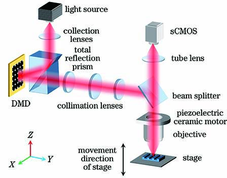
Fig. 1. Schematic of parallel differential confocal axial measurement method
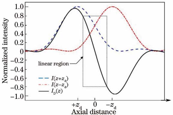
Fig. 2. Confocal axial light intensity differential response curves
Fig. 3. Schematic of calibration method of axial measurement curve
Fig. 4. Experimental platform for parallel differential confocal axial measurement
Fig. 5. Measured axial measurement curve
Fig. 6. Coin sample. (a) Actual picture and partially enlarged picture of coin sample; (b) confocal picture of coin sample in upper defocusing plane; (c) confocal picture of coin sample in lower defocusing plane
Fig. 7. Topography of coin stripes before correction. (a) Three-dimensional view; (b) top view
Fig. 8. Light intensity differential response simulation curve and axial measurement simulation curve with different peak values
Fig. 9. Light spot array images. (a) Light spot array image in focal plane; (b) enlarged view of solid line frame; (c) enlarged view of dotted line frame
Fig. 10. Axial light intensity response curves of each point in one-dimensional line
Fig. 11. Distribution diagram of light intensity peak value in global field of view
Fig. 12. Light intensity differential response curves of each point in one-dimensional line
Fig. 13. Topography of coin stripes after correction. (a) Three-dimensional view; (b) top view
Fig. 14. Three-dimensional topography of coin stripes measured using commercial microscope. (a) Three-dimensional topography of coin stripes; (b) sectional height profile curve of coin stripes
Fig. 15. Three-dimensional image inpainting figure of coin stripes. (a) Before correction; (b) after correction
Fig. 16. Sectional height profile curves of coin stripes before and after correction
Fig. 17. Step standard sample and enlarged picture of measurement position
Fig. 18. Sectional height profile curves of step standard sample before and after correction
|
Table 1. Height measurement results of standard sample step before and after correction
|
Table 2. Height error analysis of standard sample step before and after correction

Set citation alerts for the article
Please enter your email address
© Copyright 2018-2021 | Chinese Laser Press. All Rights Reserved 沪ICP备15018463号-20