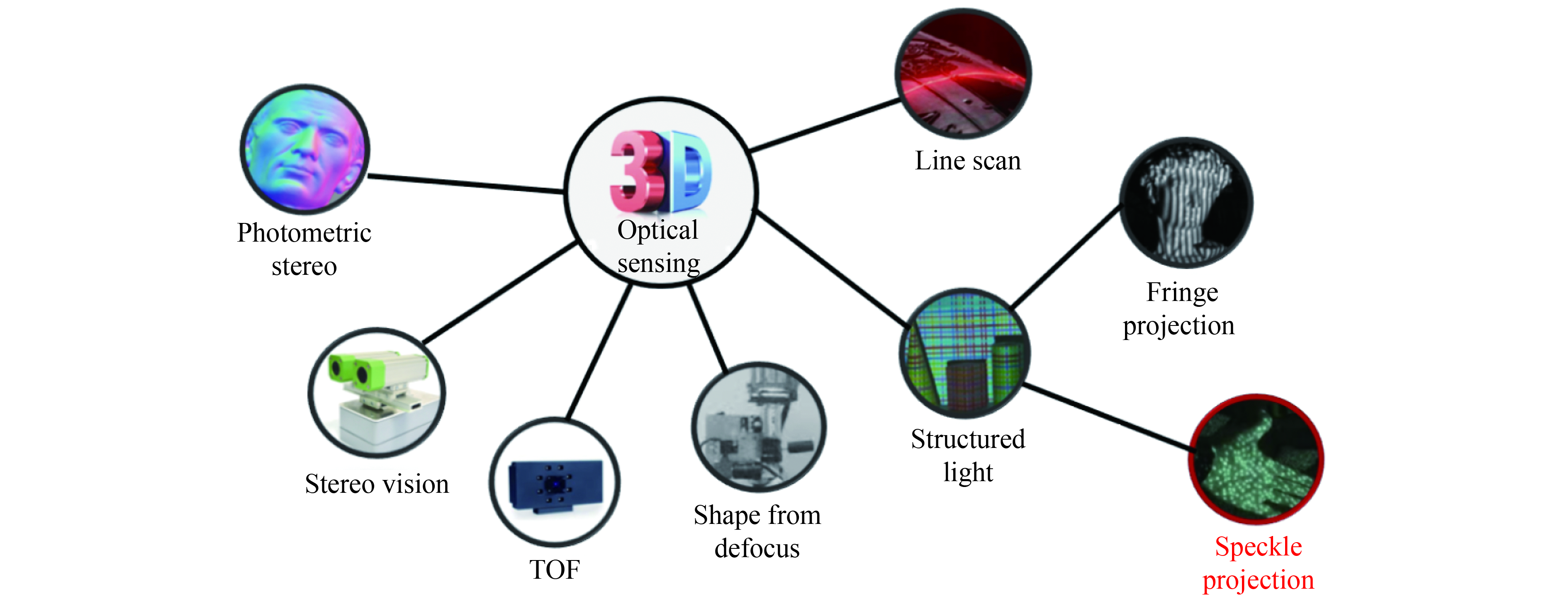
Fig. 1. Representative techniques for 3D optical sensing

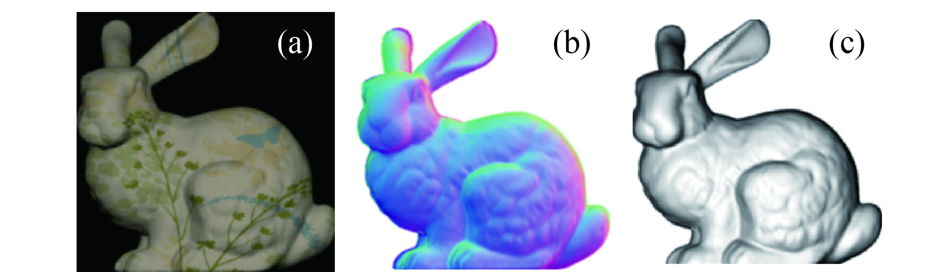
Fig. 2. Measurement results of Stanford rabbits by photometric stereo method. (a) Stanford rabbit model; (b) Normal map; (c) Reconstruction map

Fig. 3. Schematic diagram of stereo vision

Fig. 4. Schematic diagram of time-of-flight method^[24]

Fig. 5. Schematic of laser scanning

Fig. 6. Schematic diagram of defocus recovery method^[35]

Fig. 7. Measurement results of the defocus recovery method^[36]

Fig. 8. Schematic diagram of structured light projection method^[38]

Fig. 9. Fringe order ambiguity in the wrapping phase of isolated objects and discontinuity surfaces

Fig. 10. Nintendo Wii with motion sensing controller^[99]

Fig. 11. Microsoft Xbox360 with 3D motion sensor Kinect^[103]

Fig. 12. Components of Kinect and the projected speckle pattern

Fig. 13. Apple iPhone X with 3D structured light sensor^[106]

Fig. 14. Face-ID 3D face recognition technology of iPhone X^[107]

Fig. 15. Alipay and WeChat face payment terminals^[110]

Fig. 16. Ubiquitous 3D face payment terminals

Fig. 17. Schematic diagram of binocular stereo matching

Fig. 18. Difficulty in binocular matching of texture-less objects

Fig. 19. Speckle projection marks each point in space uniquely

Fig. 20. A module of an infrared structured-light 3D sensor^[118]

Fig. 21. Three semiconductor lasers models (a) VCSEL; (b) DFB EEL; (c) Fabry–Pérot EEL

Fig. 22. Emitted patterns comparison of VCSEL, LED, and EEL

Fig. 23. (a) Schematic diagram of DOE diffraction; (b) Schematic diagram of an EEL dot projector

Fig. 24. (a) Schematic diagram of DOE duplicator; (b) Schematic diagram of a VCSEL dot projector

Fig. 25. Lens wafer and a WLO lens

Fig. 26. Projected patterns based on the non-formal codification (a) slot line constraint^[43]; (b) Gray constraint^[129]

Fig. 27. Projected patterns based on De Bruijn sequences^[51] (a) De Bruijn sequences; (b) Projected patterns

Fig. 28. Projected patterns based on M-arrays^[51] (a) M-array; (b) Projected patterns

Fig. 29. Projected patterns of commercial speckle-based structured light sensors. (a) Coding method based on global uniqueness; (b) Coding method based on Sudoku; (c) Coding method based on M-array

Fig. 30. Image correlation method based on local window

Fig. 31. Principle and process of one-dimensional matching in binocular stereo vision system. (a) Basic principle; (b) Matching process

Fig. 32. Schematic diagram of matching algorithm based on reference image

Fig. 33. Schematic diagram of cost aggregation algorithm^[134]. (a) Cross construction; (b) Cost aggregation

Fig. 34. Schematic diagram of SGM^[136]. (a) Minimum cost path; (b) 16 paths from all directions

Fig. 35. Effect of local windows with different sizes on the calculation results of disparity maps

Fig. 36. Schematic diagram of triangulation measurement model based on binocular vision system

Fig. 37. Pinhole model of the camera

Fig. 38. Architecture of 3D structured light sensor

Fig. 39. Hardware architecture of 3D sensor based on customized ASIC chip^[143]

Fig. 40. Hardware architecture of 3D sensor based on FPGA^[144]

Fig. 41. Global biometric industry market share

Fig. 42. 3D face recognition using infrared ray can solve the influence of ambient illumination^[146]

Fig. 43. Face recognition based on 3D data^[148]

Fig. 44. 3D finger tracker Leap Motion

Fig. 45. Statistics of global VR/AR industry investment in 2013-2017 (Unit: USD 100 million)

Fig. 46. 3D camera space chaser N500^[154]

Fig. 47. Similarity of speckle is influenced by the 3D surface

Fig. 48. Tradeoff between global uniqueness and spatial resolution of speckle pattern

Fig. 49. Relationship between baseline distance and measurement accuracy

Fig. 50. Ideal high-precision 3D face data and real 3D face data obtained by iPhone X

Fig. 51. HD 3D mask fools face recognition systems^[155]

Fig. 52. World's first commercially mobile phone OPPO R17 Pro with ToF technology^[156]

Fig. 53. Error comparison between ToF and structured-light at different measurement depths

Fig. 54. Real-time 3D measurement system at 120 Hz for complex dynamic scene^[158]

Fig. 55. Quad-camera 3D measurement system based on SPU. (a) Appearance of the system; (b) Top view of the internal structure of the system; (c) System measurement scenario

Fig. 56. Results of the David model after registration. (a) Point cloud results; (b) Triangulation results

Fig. 57. Schematic diagram of a panoramic 3D structured light measurement system based on plane mirror reflection

Fig. 58. 3D measurement results of a Voltaire model. (a) Full-surface 3D measurement results of a Voltaire model; (b)-(d) Corresponding results of (a) from three different views

Fig. 59. Highlight intensity removal with polarizers^[205]

Fig. 60. Principle of fringe analysis method based on deep learning^[221]

Fig. 61. Basic structure of a digital projector based on Digital Light Processing (DLP) technology and its core component DMD

Fig. 62. 3D measurement and tracking a bullet fired from a toy gun. (a) Camera images at different time points; (b) Corresponding 3D reconstructions; (c) 3D reconstruction of the muzzle region (corresponding to the boxed region shown in (b)) as well as the bullet at three different points of time over the course of flight (7.5 ms, 12.6 ms, and 17.7 ms). The insets show the horizontal (x–z) and vertical (y-z) profiles crossing the body center of the flying bullet at 17.7 ms; (d) 3D point cloud of the scene at the last moment (135 ms), with the colored line showing the 130 ms long bullet trajectory. The inset plots the bullet velocity as a function of time

Fig. 63. Systems and results of 5D hyperspectral imaging and high speed thermal imaging^{[244, 245]}. (a) 5D hyperspectral imaging system; (b) High speed thermal imaging system; (c) 5D hyperspectral imaging results: the measurement of water absorption by a citrus plant; (d) High-speed thermal imaging results: the measurement of a basketball player at different times

Fig. 64. Fast 3D face scanning system FaceScan

Fig. 65. Feature points for 3D facial recognition

Fig. 66. Future world of the real “3D”

Table 1. Matching function based on cross-correlation criteria

Table 2. Matching function based on SSD-correlation criteria