
Zhiguo Zhou, Yiyao Li, Jiangwei Cao, Shunfan Di. Surface Target Detection Algorithm Based on 3D Lidar[J]. Laser & Optoelectronics Progress, 2022, 59(18): 1815006
- Laser & Optoelectronics Progress
- Vol. 59, Issue 18, 1815006 (2022)
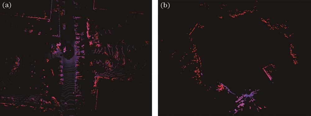
Fig. 1. Lidar point clouds in different scenes. (a) Ground point clouds; (b) calm water surface point clouds
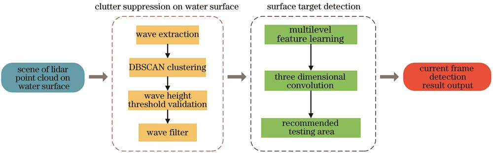
Fig. 2. Algorithm block diagram
Fig. 3. Lidar water surface echo data. (a) (b) Calm water surface; (c) (d) wave water surface
Fig. 4. DBSCAN filtering algorithm based on water surface point clouds
Fig. 5. DBSCAN clustering. (a) Wave point clouds over water; (b) clustering result
Fig. 6. Water surface target detection algorithm
Fig. 7. Structure of feature learning network
Fig. 8. VFE layer structure
Fig. 9. Region proposal network architecture
Fig. 10. Experimental platform
Fig. 11. Measured data. (a) Spheres; (b) tri-pyramid; (c) cylindrical; (d) multi-objective
Fig. 12. DBSCAN-VoxelNet loss value in the training process
Fig. 13. Construction of surface target detection simulation environment
Fig. 14. Virtual wave fluctuation state in the first view of ship
Fig. 15. Target setting of water virtual environment
|
Table 1. RS-LiDAR-16 sensor parameters
| ||||||||||||||||||||||||||||||||||||
Table 2. Detection results of DBSCAN-VoxelNet on water surface target dataset
|
Table 3. mAP detection results for water surface target
|
Table 4. mAP of DBSCAN-VoxelNet at different environments

Set citation alerts for the article
Please enter your email address
© Copyright 2018-2021 | Chinese Laser Press. All Rights Reserved 沪ICP备15018463号-20