Early-photon guided reconstruction method for time-domain fluorescence lifetime tomography

Lin Zhang; Chuangjian Cai; Yanlu Lv; Jianwen Luo

doi:10.3788/COL201614.071702

Abstract

A reconstruction method guided by early-photon fluorescence yield tomography is proposed for time-domain fluorescence lifetime tomography (FLT) in this study. The method employs the early-arriving photons to reconstruct a fluorescence yield map, which is utilized as a priori information to reconstruct the FLT via all the photons along the temporal-point spread functions. Phantom experiments demonstrate that, compared with the method using all the photons for reconstruction of fluorescence yield and lifetime maps, the proposed method can achieve higher spatial resolution and reduced crosstalk between different targets without sacrificing the quantification accuracy of lifetime and contrast between heterogeneous targets.

The fluorescence imaging technique is widely used in biological research^[1]. As a macroscopically imaging technique, fluorescence molecular tomography (FMT) has great potential in the early diagnosis of disease, etc^[2]. Many methods have been developed to improve the reconstruction quality^[3] and reduce the computational cost of FMT^[4]. The fluorescent targets embedded in biological tissue can be described by fluorescence yield and fluorescence lifetime. Fluorescence yield can be acquired by continuous-wave mode FMT, frequency-domain mode FMT, or time-domain (TD) mode FMT, while fluorescence lifetime can be obtained by the latter two modes. For specific kinds of fluorochromes, fluorescence lifetime is environmentally sensitive. In other words, it is easily influenced by tissue oxygenation, temperature, and so on^[5]. So, fluorescence lifetime tomography (FLT) can expand and optimize the application of FMT. For example, FLT can help observe fluorescence response energy transfer in vivo^[6].

As a particular strategy of TD FMT, the time-gate technique using early-arriving photons which undergo few scattering events has been validated to provide a high spatial resolution in the reconstruction of fluorescence density^[7,8].

In recent years, more and more studies on fluorescence lifetime imaging have been performed. With fluorescence lifetime as a known feature of the measured dataset, the yields of multitudinous lifetime components can be obtained^[9], and high special resolution and lifetime contrast are achieved for closely located targets^[10]. For FLT, Laplace transform^[11,12] and Fourier transform^[13] are utilized to obtain the lifetime of fluorescent targets deep in a turbid medium, and the key point is to reduce the complexity brought by temporal convolution. Recently, our group proposed a direct reconstruction method for TD FLT (DFLT for short) via a nonlinear optimized fitting procedure^[14]. In the DFLT method, the fluorescence yield map, reconstructed by a method similar to that used in the continuous-wave mode, is employed as a priori information, and L1 (L1 norm, which denotes the sum of the absolute value of each element of a vector) regularization is employed to obtain the fluorescence lifetime map. The DFLT method provides high localization accuracy for fluorescent targets, high quantification accuracy for fluorescence lifetime, and good contrast between targets that are not very closely located. However, the crosstalk between targets is non-negligible, and for targets embedded more closely, the quantification accuracy and contrast are reduced.

Sign up for Chinese Optics Letters TOC. Get the latest issue of Chinese Optics Letters delivered right to you！Sign up now

Considering the benefits of the time-gate technique, an early-photon guided reconstruction method for TD FLT (EPFLT for short) is proposed in this Letter. This method employs the reconstruction results of fluorescence yield from early-arriving photons to achieve a higher spatial resolution, and utilizes all the measurement data to fit the lifetime for the targets on the early-photon yield map. By using this method, the crosstalk between the different targets is significantly reduced without sacrificing the high quantification accuracy and good contrast, even for the more closely located targets.

The telegraph equation is used to describe photon propagation for both excitation light and emitted fluorescence^[15], $\frac{D (r)}{c^{2}} \frac{\partial Φ_{x, m}^{2} (r, t)}{\partial t} + \frac{1}{c} (3 D (r) μ_{a} + 1) \frac{\partial Φ_{x, m} (r, t)}{\partial t} + μ_{a} Φ_{x, m} (r, t) - \nabla \cdot [D (r) \nabla Φ_{x, m} (r, t)] = s_{x, m} (r, t),$ (1)where $Φ_{x, m} (r, t)$ denotes the excitation and emission photon density at location $r$ and time $t$ , $D (r)$ is the diffusion coefficient defined by $D (r) = 1 / (3 (μ_{a} + μ_{s}^{'}))$ , $μ_{a}$ is the absorption coefficient, and $μ_{s}^{'}$ is the reduced scattering coefficient. The source term for excitation is $s_{x} (r, t) = δ (r - r_{s}, t)$ , while the source term for emission is $s_{m} (r, t) = Φ_{x} (r, t) * \exp (- t / τ (r)) η (r) / τ (r)$ , where $*$ stands for the temporal convolution operator.

The fluorescence signal $Φ_{m}$ measured at a detect point $r_{d}$ for an excitation source at point $r_{s}$ , referred to as the temporal-point spread function (TPSF), can be written as ${\begin{cases} Φ_{m} (r_{d}, r_{s}, t) = \int_{Ω} w (r, r_{d}, r_{s}, t) * \exp (- \frac{t}{τ (r)}) \frac{η (r)}{τ (r)} d^{3} r \\ w (r, r_{d}, r_{s}, t) = G_{m} (r, r_{d}, t) * Φ_{x} (r_{s}, r, t) \end{cases},$ (2)where $w (r, r_{d}, r_{s}, t)$ is the weight matrix, and $G_{m} (r, r_{d}, t)$ is the Green’s function of the emission light.

In order to solve Eq. (1), the Galerkin finite element method (FEM) is utilized to obtain the temporal recursion matrix equation, while an implicit finite difference scheme^[16] is adopted to approximate the time derivatives. Then the imaging domain is discretized into a three-dimensional (3D) mesh with $N_{v}$ ( $N_{v} = N_{x} \times N_{y} \times N_{z}$ , where $N_{x}$ , $N_{y}$ , and $N_{z}$ denote the number of elements along the $x$ axis, $y$ axis, and $z$ axis, respectively) nodes with a volume of each voxel of the grid $Δ V$ , and the time sequence is discretized by a time interval $Δ t$ .

A fluorescence yield map reconstructed from the early-arriving photons is needed first. As early-arriving photons offer poor lifetime sensitivity^[11], the lifetime $τ (r)$ is set to be a constant $τ_{0}$ invariant with $r$ to obtain the yield map. The preset constant $τ_{0}$ is obtained from the late-arriving (i.e., declining) part of the measured TPSFs by least-squares approximation. By employing the Born normalization method^[17], the forward problem for the time-gate technique is written as ${\begin{cases} Φ_{m} (r_{d}, r_{s}, t_{gate}) = \int_{Ω} W^{n} (r, r_{d}, r_{s}, t_{gate}) η (r) d^{3} r \\ W^{n} (r, r_{d}, r_{s}, t_{gate}) = \frac{{[w (r, r_{d}, r_{s}, t) * \exp (- t / τ_{0})]}_{t = t_{gate}}}{Φ_{x} (r_{s}, r, t_{gate})} \end{cases} .$ (3)

To obtain a reasonable solution, the Tikhonov regularization is usually adopted to acquire the optimization function^[3]: $R η = \arg \min_{η \geq 0} {‖ W^{n e} R η - Φ_{m e} ‖}_{2}^{2} + λ {‖ I η ‖}_{2}^{2},$ (4)where $R η (r)$ is the early-photon based yield map to be reconstructed, $λ$ is the regularization parameter, and $I$ is an identity matrix. The optimization problem is solved by the projected restarted conjugate gradient normal residual algorithm^[3].

The reconstructed yield map $R η (r)$ is then utilized as a priori information for the reconstruction of FLT. To reduce the influence of the preset lifetime $τ_{0}$ and to make use of the early-photon based yield map, both sides of the first equation in Eq. (2) are integrated with respect to $t$ , resulting in the following equation: $\int_{0}^{t} Φ_{m} (r_{d}, r_{s}, t) d t = \int_{Ω} W (r, r_{d}, r_{s}, t) η (r) d^{3} r - \int_{Ω} w (r, r_{d}, r_{s}, t) * \exp (- t Γ (r)) η (r) d^{3} r,$ (5)where $W (r, r_{d}, r_{s}, t)$ is the time integration of $w (r, r_{d}, r_{s}, t)$ , and the lifetime $τ (r)$ is replaced by the inverse lifetime $Γ (r)$ ( $Γ (r) = 1 / τ (r)$ ) to avoid dealing with the singularity of the zero points in the lifetime image.

By replacing the fluorescence yield $η (r)$ with the yield map $R η (r)$ which has been reconstructed from the early-arriving photons, replacing the expression $\int_{0}^{t} Φ_{m} (r_{d}, r_{s}, t) d t$ with the symbol $Y_{m}$ , and replacing the expression $\int_{Ω} W (r, r_{d}, r_{s}, t) η (r) d^{3} r$ with the symbol $R ϕ_{m}$ , Eq. (5) can be modified to $R ϕ_{m} (r_{d}, r_{s}, t) - Y_{m} (r_{d}, r_{s}, t) = \int_{Ω} w (r, r_{d}, r_{s}, t) * \exp (- t Γ (r)) R η (r) d^{3} r,$ (6)where $R ϕ_{m}$ can be calculated directly, and $Y_{m}$ is the measurement data. To ensure that the left side of Eq. (6) is non-negative ( $R ϕ_{m} (r_{d}, r_{s}, t) \geq Y_{m} (r_{d}, r_{s}, t)$ ), the cumulative TPSF $Y_{m} (t)$ for each source-detector pair is normalized by the maximum value of $R ϕ_{m} (t)$ , i.e., $R ϕ_{m} (t) | t = t_{end}$ , and the normalization is carried out according to the following equation: $Y_{m} (r_{d}, r_{s}, t) = Y_{m} (r_{d}, r_{s}, t) / Y_{m} (r_{d}, r_{s}, t_{end}) \times R ϕ_{m} (r_{d}, r_{s}, t_{end}) .$ (7)

After that, the relationship between the rearranged measurement sequence and the inverse lifetime can be simplified as the following nonlinear matrix equation: $R Φ = f (Γ) .$ (8)

Because the source number is $S$ , the detector number is $D$ , and the length of the time sequence discretized by the time interval $Δ t$ is $T$ , the rearranged measurement vectors $R Φ$ has $S \times D \times T$ elements, the discretized weight matrix $W$ has $S \times D \times T$ rows and $N_{v}$ columns, and the length of the yield map $R η$ reconstructed from the early-photons is $R Φ$ . The $i$ th ( $1 \leq i \leq S \times D \times T$ ) element of $R Φ$ is given by $R Φ_{i} = f {(Γ)}_{i} = \sum_{n = 1}^{N_{v}} Δ V R η (n) {[w (n, d_{i}, s_{i}, t) * \exp (- t \cdot Γ (n))]}_{t = t_{i}} .$ (9)

As $\nabla R Φ$ is the gradient matrix of $R Φ$ , the $i$ th element of $\nabla R Φ$ is shown as, $\nabla R Φ_{i} = \sum_{n = 1}^{N_{v}} Δ V R η (n) Γ (n) {[w (n, d_{i}, s_{i}, t) * \exp (- t \cdot Γ (n))]}_{t = t_{i}} .$ (10)

The optimization function is generated to obtain the stable solution: $Γ = \arg \min_{Γ > 0} ({‖ f (Γ) - R Φ ‖}_{2}^{2} + α \sqrt{{‖ Γ ‖}_{2}^{2} + β}),$ (11)where $α$ is the regularization parameter, and $β$ is the positive smooth parameter.

Similar to the DFLT method, the optimization function is solved by a back-tacking linear search based nonlinear conjugate gradient method^[18].

In summary, the proposed EPFLT method can be implemented by four steps. First, a preset of the lifetime $τ_{0}$ is obtained with a least-squares approximation from the late-arriving photons. Second, assuming that the lifetime has the same value $τ (r) = τ_{0}$ for all locations $r$ in the imaging domain, the yield map $R η (r)$ is reconstructed from the early-arriving photons. Third, the modified measured sequence $R ϕ_{m}$ is calculated and normalized with the yield map $R η (r)$ and the integrated weight matrix $W (r, r_{d}, r_{s}, t)$ to obtain the rearranged forward problem for lifetime reconstruction. Finally, a nonlinear optimization function of the inverse problem is obtained to reconstruct the inverse lifetime map $Γ (r)$ , from which the lifetime $τ (r)$ is calculated.

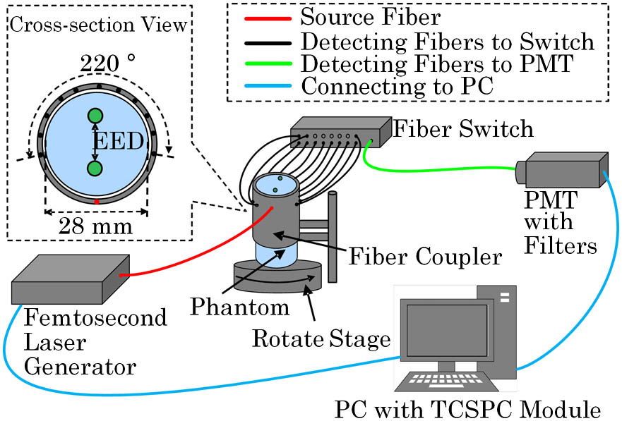
The measurements are acquired on a fiber-coupled, time-correlated single-photon-counting (TCSPC) based TD system, schematically depicted in Fig. 1. The excitation source is an ultrafast laser generated by a femtosecond laser generator (Spectra-Physics, Newport Corporation, Irvine, CA, USA) working at the wavelength of 775 nm. A cylindrical phantom with an inner diameter of 28 mm is filled with a 1% intralipid solution and is fixed on a rotation stage. The transmitted light, referred to as the TPSF, passes through a fluoresence filter ( $840 \pm 6 nm$ bandpass, ff01-840/12-25, Semrock, USA) and is detected by a multi–anode photomultiplier (PMT) (PML-16-C, Becker & Hickl GmbH, Germany) via fibers coupled to a hollow cylindrical fiber coupler and a $16 \times 1$ switch. When the stage rotates, the phantom moves together while the fiber coupler and fibers keep still. Then the detected TPSF is processed by the TCSPC module (SPC-150, Becker & Hickl GmbH, Germany). For each source-detector pair, the acquisition time is 10 s and about $1 \times 10^{6}$ photons are collected.

Figure 1.Schematic of the measurement system.

As the fluorescent targets, two cylindrical tubes (4 mm in diameter and 8 mm in height) filled with the solution of indocyanine green (ICG) are embedded in the phantom. During the experiments, the phantom is rotated over 360° in 20° increments, so the measurement data consist of 18 projections ( $S = 18$ ). For each projection, there are 11 detection points ( $D = 11$ ), and the interval of each two is set to 20°, so that the field of view of detection is 220°.

The time-gate for the early-photon is chosen to be 600 ps to hold the advantage of the early-photon technique and reduce the influence of noise. The regularization parameter is chosen to be $1 \times 10^{- 2}$ for early-photon based reconstruction and $1 \times 10^{- 19}$ for lifetime reconstruction. Both regularization parameters are chosen experientially and generally fit to the L-curve^[19]. The length of the time sequence for reconstruction is 100 ( $T = 100$ ) with an interval of 50 ps.

Four experiments (Expts. 1–4) are carried out to validate the proposed method. In the first two experiments, the edge-to-edge distance (EED) between the two homogeneous targets (Expt. 1) or heterogeneous targets (Expt. 2) is 9 mm. In the second two experiments, the EED between the two homogeneous targets (Expt. 3) or heterogeneous targets (Expt. 4) is 5 mm. In the homogeneous experiments, both cylindrical tubes are filled with 10 μmol/L of solution of ICG/dimethyl sulphoxide (ICG/DMSO), which has been measured to be 0.97 ns in the lifetime^[20]. In the heterogeneous experiments, one tube is filled with 10 μmol/L of solution of ICG/DMSO, and the other one is filled with 10 μmol/L of solution of ICG/absolute alcohol (ICG/ALC), which has been measured to be 0.62 ns in the lifetime^[20]. The approximate lifetimes $τ_{0}$ for the early-photon yield reconstruction of the four experiments are 1.74, 2.21, 1.97, and 2.09 ns, respectively.

Figure 2 shows the inverse lifetimes $Γ (r)$ of Expt. 1 and 2 ( $EED = 9 mm$ ) reconstructed by the EPFLT method and the DFLT method, respectively. The peak values of the two fluorescent targets are regarded as the reconstructed inverse lifetimes ( $Γ_{1}$ and $Γ_{2}$ ). The lifetimes of the two targets $τ_{n}$ are calculated as $τ_{n} = 1 / Γ_{n}$ ( $n = 1$ , 2).

Figure 2.Reconstruction results of (a) and (b) Expt. 1 and (c) and (d) Expt. 2. (a) and (c) denote the inverse lifetime maps obtained by the EPFLT method, while (b) and (d) denote those obtained by the DFLT method. The red and green circles denote the phantom border and the position of fluorescence targets, respectively.

The inverse lifetime maps of Expts. 3 and 4 ( $EED = 5 mm$ ) reconstructed by the EPFLT method and the DFLT method are shown in Fig. 3, respectively.

Figure 3.Reconstruction results of (a) and (b) Expt. 3 and (c) and (d) Expt. 4. (a) and (c) denote the inverse lifetime maps obtained by the EPFLT method, while (b) and (d) denote those obtained by the DFLT method. The red and green circles denote the phantom border and the position of fluorescence targets, respectively.

Figures 2 and 3 demonstrate that the EPFLT method provides a higher spatial resolution than the DFLT method.

The profiles along the dashed–dotted lines in Figs. 2 and 3 demonstrate qualitatively the performance of the EPFLT and DFLT methods in spatial resolution and localization accuracy, as shown in Fig. 4.

Figure 4.Profiles along the dashed-dotted lines in Figs. 2 and 3 for (a) Expt. 1, (b) Expt. 2, (c) Expt. 3, and (d) Expt. 4. The red lines denote the real inverse lifetime profiles, while the blue and green lines denote the inverse lifetime results obtained by the EPFLT and DFLT methods, respectively.

With $τ_{rec}$ denoting the reconstructed lifetime, $τ_{real}$ denoting the real lifetime, and $τ_{cross}$ denoting the value of the crosstalk between the two targets, the relative error (RE, $RE = | τ_{rec} - τ_{real} | / τ_{real} \times 100 %$ ) of the reconstructed lifetime and the real lifetime, the relative difference (RD, $RD = | τ_{rec 1} - τ_{rec 2} | / \min {τ_{rec 1}, τ_{rec 2}} \times 100 %$ ) of lifetimes between the two targets, and the relative crosstalk (RC, $RC = Γ_{cross} / \min {Γ_{rec 1}, Γ_{rec 2}} \times 100 %$ ) value between the two targets are used to quantitatively evaluate the performance of the different methods. The contrast-to-noise ratio (CNR, $CNR = (Γ_{T} - Γ_{B}) / {(w_{T} σ_{T}^{2} + w_{T} σ_{B}^{2})}^{1 / 2}$ ) is also used to evaluate the quality of the reconstructed image^[21], where $Γ_{T}$ and $Γ_{B}$ denote the mean values in the regions of the fluorescence targets and the background, $w_{T}$ and $w_{B}$ are weighting factors determined by the relative volumes of the corresponding regions, and $σ_{T}^{2}$ and $σ_{B}^{2}$ are the variances in the regions of the fluorescence targets and the background, respectively. The evaluation results are shown in Tables 1 and 2.

Expt.	Solvent	τEP(ns)	τD(ns)	Real lifetime (ns)	REEP (%)	RED (%)
1	DMSO	0.874	1.068	0.97	9.9	10.1
1	DMSO	0.942	1.037	0.97	2.9	6.9
2	DMSO	0.827	0.843	0.97	14.7	13.1
2	ALC	0.652	0.640	0.62	5.2	3.2
3	DMSO	1.022	1.019	0.97	5.4	5.0
3	DMSO	0.998	0.993	0.97	2.9	2.4
4	DMSO	0.902	1.067	0.97	7.0	10.0
4	ALC	0.672	0.853	0.62	8.4	37.5

Table 1. Comparison of Fluorescence Lifetimes and Relative Errors by the EPFLT and DLFT Methods

View all Tables

Expt.	Method	CNR	RD (%)	Real RD (%)	RC (%)
1	EPFLT	7.37	7.8	0	0
1	DFLT	2.38	3.0	0	46.6
2	EPFLT	6.00	26.8	56.45	0
2	DFLT	2.30	31.7	56.45	53.8
3	EPFLT	4.45	2.4	0	0
3	DFLT	2.65	2.0	0	63.5
4	EPFLT	4.39	34.2	56.45	0
4	DFLT	2.44	8.5	56.45	77.7

Table 2. Comparisons of Contrasts and Crosstalks

View all Tables

Table 1 compares the lifetimes and the Res obtained by the EPFLT and DFLT methods. $τ_{EP}$ denotes the lifetime reconstructed by the EPFLT method, and $τ_{D}$ denotes that by the DFLT method. ${RE}_{EP}$ and ${RE}_{D}$ denote the Res by the EPFLT and DFLT methods, respectively. All the Res of lifetime reconstructed by the EPFLT method are below 15% ( ${RE}_{EP}$ ). The DFLT method provides high quantification accuracy in the fluorescence lifetime for homogeneous targets (Expts. 1 and 3) and heterogeneous targets with an EED of 9 mm (Expt. 2), but fails in obtaining accurate reconstruction for heterogeneous targets with an EED of 5 mm (Expt. 4).

The quantitative results of CNR, RD, and RC are shown in Table 2, where Real RD denotes the RD of the real lifetime. The targets reconstructed by the EPFLT method can be separated without crosstalks ( $RC = 0$ ). However, the crosstalks of the DFLT results are non-negligible because of the high RC values. According to the values of RD, the EPFLT and DFLT method performs well in terms of quantification accuracy and contrast of target with a different fluorescence lifetime for experiments with an EED of 9 mm (Expts. 1 and 2). For heterogeneous targets with a smaller EED (Expt. 4), the EPFLT method can still provide accurate quantification of the fluorescence lifetime, while the DFLT has larger REs. Comparing the two methods, the variation of CNR is consistent with that of the resolution, which demonstrates that the EPFLT method can provide a higher reconstruction quality.

In conclusion, an early-photon guided reconstruction method is proposed for TD FLT in this Letter. The proposed method benefits from the early-photon technique, which can offer a higher spatial resolution yield map for FLT and has an advantage in the location accuracy. To reduce the influence of approximate lifetime, the inverse problem is transformed by integration and normalization. Results of the phantom experiments demonstrate that the proposed method can provide accurate quantification of lifetime, relatively high localization accuracy, good contrast in lifetime, and improved spatial resolution compared to the DFLT method. However, although early-arriving photons can offer higher spatial resolution and localization accuracy, they are very small in amount and are easily disturbed by the system noise, especially when the fluorescent targets are very deeply embedded. As a result, there is noise along the border in the reconstructed maps. In the future, a more effective early-gate technique and a system with low noise will be developed to improve the results.

References

[1] Y. He, Z. Wang, Y. Wang, L. Wei, X. Li, J. Yang, G. Shi, Y. Zhang. Chin. Opt. Lett., 13, 111702(2015).

[2] V. Ntziachristos, J. Ripoll, L. V. Wang, R. Weissleder. Nat. Biotechnol., 23, 313(2005).

[3] X. Cao, B. Zhang, F. Liu, X. Wang, J. Bai. Opt. Lett., 36, 4515(2011).

[4] J. Zhang, J. Shi, S. Zuo, F. Liu, J. Bai, J. Luo. Chin. Opt. Lett., 13, 071002(2015).

[5] M. A. O’Leary, D. A. Boas, X. D. Li, B. Chance, A. G. Yodh. Opt. Lett., 21, 158(1996).

[6] J. M. Ginty, D. W. Stuckey, V. Y. Soloviev, R. Laine, M. Wylezinska-Arridge, D. J. Wells, S. R. Arridge, P. M. W. French, J. V. Hajnal, A. Sardini. Biomed. Opt. Express, 2, 1907(2011).

[7] M. Niedre, V. Ntziachristos. Opt. Lett., 35, 369(2010).

[8] B. Zhang, X. Cao, F. Liu, X. Liu, X. Wang, J. Bai. Appl. Opt., 50, 5397(2011).

[9] A. T. N. Kumar, S. B. Raymond, G. Boverman, D. A. Boas, B. J. Bacskai. Opt. Express, 14, 12255(2006).

[10] S. S. Hou, W. L. Rice, B. J. Bacskai, A. T. N. Kumar. Opt. Lett., 39, 1165(2014).

[11] F. Gao, W. Liu, H. Zhao. Chin. Opt. Lett., 4, 595(2006).