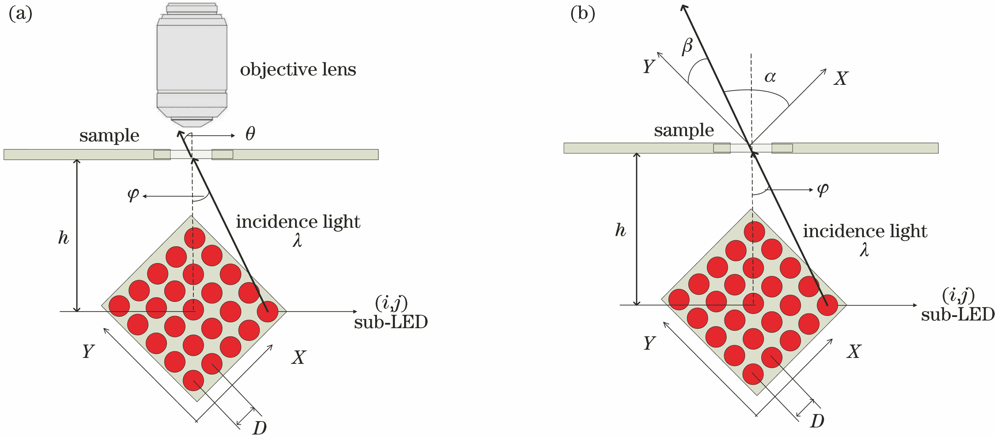
Fig. 1. Spatial position relationship in the setup. (a) Spatial position relationship and basic light path of the setup; (b) specific light path with edge rays

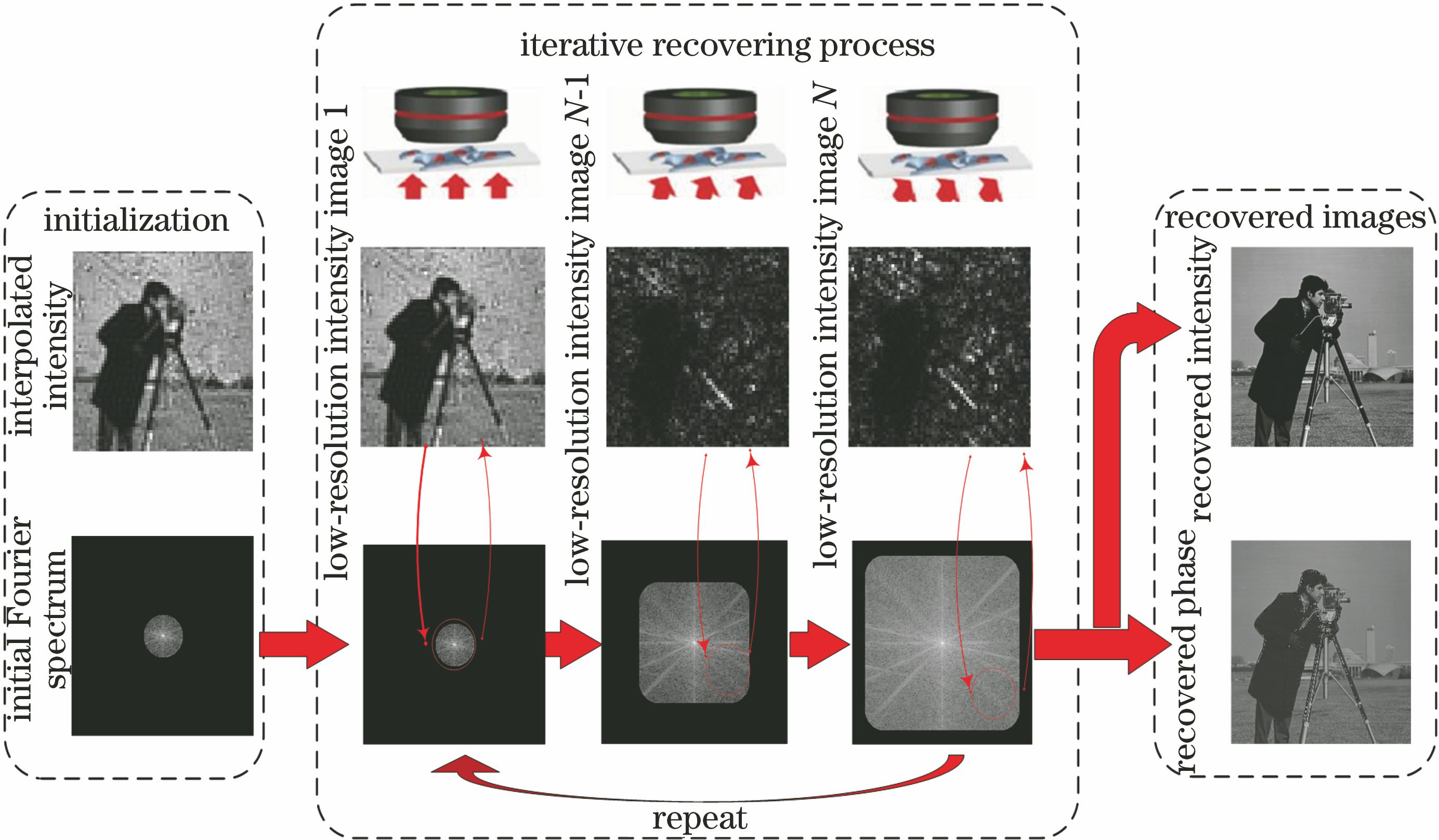
Fig. 2. Recovery process of FPM

Fig. 3. Sketch map of synthetic aperture for full spectrum after spectrum extension

Fig. 4. Tested images. (a) Man; (b) coin; (c) icon; (d) rice; (e) X-ray image; (f) tire; (g) target; (h) aerial view; (i) text; (j) flower

Fig. 5. D_φ1 of SSIM corresponding to each image of Fig. 4. (a) Man; (b) coin; (c) icon; (d) rice; (e) X-ray image; (f) tire; (g) target; (h) aerial view; (i) text; (j) flower

Fig. 6. D_φ2 of PSNR corresponding to each image of Fig. 4. (a) Man; (b) coin; (c) icon; (d) rice; (e) X-ray image; (f) tire; (g) target; (h) aerial view; (i) text; (j) flower

Fig. 7. Selection method of most important LEDs following the principle of area of rhombus and four corners

Fig. 8. Comparisons of simulated results under different patterns of LED angle illumination. (a1)(a2) Original input amplitude and phase of the high-resolution object, (d1)(d2) the partial enlargement of amplitude image; (b1)(b2) recovered complex amplitude (amplitude and phase) with conventional lighting one by one using 225 LEDs, (e1)(e2) the partial enlargement of amplitude image; (c1)(c2) recovered complex amplitude (amplitude and phase) with using 57 LEDs, (f1)(f2) the partial enlargement of amplit

Fig. 9. Setup and optical path of proposed method. (a)Setup; (b) optical path

Fig. 10. Comparisons of experimental results under different patterns of LED angle illumination. (a) Raw data with the vertical incidence LED (the central LED) and its local magnification; (b) recovered amplitude with conventional lighting one by one using 225 LEDs and its local magnification; (c) recovered amplitude with proposed method (only using 57 LEDs) and its local magnification; (d) intensity curves of the local map of the central area

Fig. 11. Comparisons of experimental results under different patterns of LED angle illumination. (a) Raw data with the vertical incidence LED (the central LED); (b) local magnification; (c1)(c2) recovered amplitude and recovered phase with conventional lighting one by one using all 225 LEDs; (d1) (d2) recovered amplitude and recovered phase with our strategy (only using 57 LEDs)

Table 1. Comparison of objective evaluation indexes for amplitude comparison of Fig. 8(b1) and (c1)

Table 2. Comparison of objective evaluation indexes for amplitude comparison of Fig. 8(e1), (e2), (f1), and (f2)

Table 3. Comparison of objective evaluation indexes and efficiencies for Fig. 10